|
| ||
Step 1: |
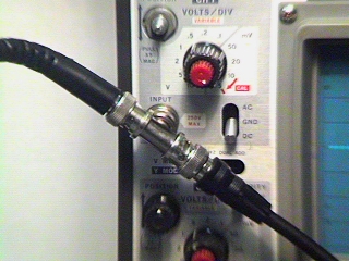
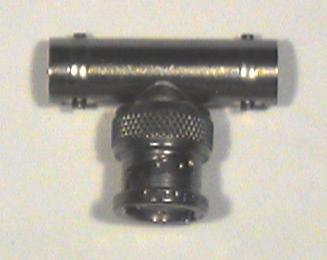
Connect your
BNC T connector
to
CH1
of the scope.
| |
Step 2: |
Use a BNC patch cord to connect one end of the T to the
function generator output.
Connect a BNC clip lead to the other end of the T.
| |
Step 3: |
Set the function generator to produce a
2 V p-p (i.e. 1 V peak),
100 Hz sine wave.
| |
Step 4: |
Set the DMM to
AC Volts
and connect the probes to the clip leads.
What is the voltage reading on the DMM?
| |
Step 5: |
Set the function generator to produce a square wave.
Readjust the
Amplitude
control if necessary to maintain the
2 V p-p amplitude.
What is the voltage reading on the DMM?
| |
Step 6: |
Reset the function generator to sine wave.
Note the reading on the DMM at
5 Hz,
50 Hz,
500 Hz,
5 kHz,
and 50 kHz.
| |
Question 1: |
What is the useful frequency range of the DMM for
measuring AC signals?
| |
Diversion: |
The AC voltage function of the DMM is calibrated
to read (approximately) the
RMS
value of the waveform.
RMS stands for root-mean-square
i.e. the square root of the mean value of the square of the function:
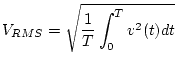
We'll see the importance of this when we study power.
For now, just remember that for a sine wave,
|
| |||
Step 1: |
Wire the following circuit, using 10k![\includegraphics[scale=0.650000]{ckt3.1.1.ps}](img162.png)
What should the divider ratio ( | ||
Step 2: |
Set the function generator to produce a 2 V p-p
sine wave.
| ||
Step 3: |
Using the oscilloscope,
measure | ||
Step 4: |
Without disturbing the function generator settings,
replace the two 10k | ||
Step 5: |
Again leaving the function generator alone,
replace both resistors with
1M | ||
Moral: |
No circuit exists in isolation.
To be useful its input or output (or both) must be connected
to some other circuit.
Unfortunately, the interaction between the circuit and a non-ideal
source or load
causes it to behave differently than it would in an idealized
situation.
With careful design, this interaction can be
minimized or accounted for.
If ignored it can reduce the performance of the
system, or keep it from working altogether.
For example, for the measurements we made in this part, we would have the following model for the complete system including circuit, source, and load: ![\includegraphics[scale=0.400000]{ckt3.1.2.ps}](img163.png)
| ||
Question 2: |
Based on your measurements and the above model,
what are the output resistance ( |
A
potentiometer
(or
pot
for short)
is a fixed value resistor with a third, movable contact
or
slider
which may be positioned anywhere along the
resistive element.
If we represent the position of the slider by
![]() , where
, where ![]() varies between 0 (fully counterclockwise)
and 1 (fully clockwise), then the resistance between the lower
end of the resistor and the slider will be
varies between 0 (fully counterclockwise)
and 1 (fully clockwise), then the resistance between the lower
end of the resistor and the slider will be ![]() and between
the slider and the upper end will be
and between
the slider and the upper end will be ![]() ,
where
,
where ![]() is the total resistance of the potentiometer.
is the total resistance of the potentiometer.
If we connect the two fixed contacts to a voltage source and measure the output between the movable contact and one fixed contact, we get a variable voltage divider:
![\includegraphics[scale=0.650000]{pot1.ps}](img164.png)
Then the output is
|
| |||
Step 1: |
Select a 10k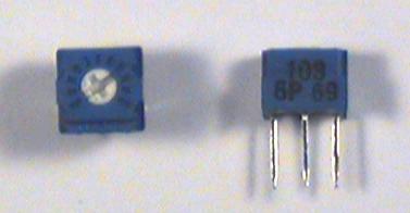
| ||
Step 2: |
Wire the following circuit:
![\includegraphics[scale=0.650000]{ckt3.1.3.ps}](img165.png)
| ||
Step 3: |
Set the function generator to produce a
2 V p-p
100 Hz sine wave.
| ||
Step 4: |
Set the potentiometer adjustment screw to mid scale
and measure | ||
Step 5: |
The potentiometer has a scale divided into 10 equal divisions,
presumably representing 10 equal divisions of resistance.
Set the potentiometer to each of these 10 divisions and measure
|
If in the volume control circuit above,
![]() were fixed at
were fixed at ![]() and
and ![]() varied with time,
we would have
varied with time,
we would have
![]() ,
i.e. we would have a
resistive transducer.
More common is where we have just a single resistor
with
,
i.e. we would have a
resistive transducer.
More common is where we have just a single resistor
with ![]() , where
, where ![]() is the physical parameter being
measured.
is the physical parameter being
measured.
For example, if ![]() represents the acoustical pressure
in a sound wave and we have a resistance which varies with
pressure,
represents the acoustical pressure
in a sound wave and we have a resistance which varies with
pressure, ![]() ,
then in the following circuit we would have
,
then in the following circuit we would have
![]() ,
where
,
where ![]() .
.
![\includegraphics[scale=0.650000]{ckt3.1.4a.ps}](img166.png)
The output consists of the desired signal,
![]() ,
superimposed on a constant DC offset,
,
superimposed on a constant DC offset, ![]() .
We saw this last week with the photodiode, and we know
how to deal with this offset: just switch the scope to
AC.
.
We saw this last week with the photodiode, and we know
how to deal with this offset: just switch the scope to
AC.
|
| ||
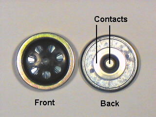
Step 1: |
Unscrew the cover from the mouthpiece of the telephone handset.
Carefully remove the microphone cartridge.
| |
Step 2: |
Shake or tap the microphone and measure | |
Step 3: |
Replace the microphone in the handset and replace the cover.
| |
Diversion 1: |
Since we don't have any current sources in the lab,
we'll have to build an approximate current source
the way we talked about in class:
by connecting a voltage source in series with a large resistor.
When we do, we get the following circuit
(which looks suspiciously like a voltage divider):
![\includegraphics[scale=0.650000]{ckt3.1.4b.ps}](img167.png)
| |
Diversion 2: |
In the last two Labs we used the 0-6V half of the power supply
as a signal source.
We will be using the other half ( | |
Step 4: |
Connect the
GND
and
+15V
connector blocks to two rows on
the top bus strip.
Connect the gaps at the center of the bus strip to form two
full width power buses.
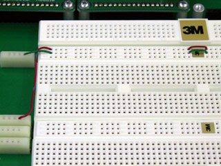
You now have a power and ground bus that looks like this: ![\includegraphics[scale=0.650000]{pwr_bus1.ps}](img168.png)
| |
Step 5: |
Set the
Meter Selector
switch on the power supply to
+20V.
Adjust the
0 to 20V
voltage control to product 10 volts.
| |
Step 6: |
Use a red banana patch cord to connect the
0 to +20V
terminal of the power supply to the red banana jack on the breadboard.
With a green cord, connect the
Common
terminal to the green banana jack.
| |
Step 7: |
Plug one end of a
handset coil cord
into the handset
and the other end into J1-7 of the interface board.
| |
Step 8: |
Connect one side of the microphone to ground by
connecting pin 13 (mic2) of the interface board socket strip to
pin 14 (gnd).
Plug the other side of the microphone (pin 12)
into a hole in the breadboard socket strip.
| |
Step 9: |
Into another hole in the same column,
plug one end of a 4.7 k | |
Step 10: |
We now should have wired the circuit shown in the figure above.
Connect
CH1
of the oscilloscope to 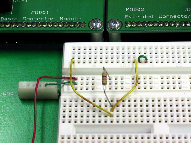
| |
Step 11: |
Speak into microphone and observe | |
Question 3: |
How does the signal amplitude of the carbon microphone compare with that of the microphone we used last week? Could we connect this directly to the speaker or handset earpiece and produce an audible sound? |