Introduction
Variables
Functions
Plotting
Tutorial videos
Variables have names conforming to the usual programming conventions, and are case sensitive (names a and A refer to different variables). Variables contain matrices (a rectangular array of numbers). To set x to be a vector of the first five integers, you type
>> x = [1 2 3 4 5];
(>> is Matlab's prompt for the next command). The square brackets define the quantities within a matrix. Element of the matrix can be a number (as in this example) or an expression like
>> x = [1 1+1 4-1 12/3 5^1];
Addition, subtraction, multiplcation and division are representd by the usual symbols. ^ means exponentiation. The semicolon at the end of the line tells Matlab that you don't what it to display the contents of the variable you're setting. To initialize a variable to be a 2x3 matrix (two rows and three columns), you would type something like
>> A = [1 2 3;4 5 6]
to which Matlab responds with
A =
1 2 3
4 5 6
Going back to the row vector example, defining a variable to be a sequence of numbers can be done two ways: by typing them in (this could be tedious; how about the first 100 integers!) or by using the colon notation. Here, [b:s:e] means the vector
[b:s:e] means [b b+s b+2*s ... e]
b means the beginning value, s the step between values, and e the ending value (the last entry may not equal e; the exact value equals the largest value of b+n*s that's less than or equal to e). Our example could be much more consisely written
>> x = [1:5];
Note that when the step is 1, you don't have to specify it. Note that if you wanted a vector starting at 0, stepping by 0.01, and going to 1, you can do that two ways.
>> x = [0: 0.01: 1];
or
>> x = .01*[0:100];
For geometrically increasing steps, as is appropriate for frequency variables to be plotted on logarithmic coordinates, use the function logspace.
f = logspace(e1, e2, n) creates a length-n vector whose values increase geometrically from 10e1 to 10e2.
You can add and subtract variables so long as they are the same size matrices. * and / refer to matrix multiplication and a form of matrix division; in these case, variable sizes must conform to the usual matrix conventions. Matlab has the special operators .* and ./ that perform term-by-term multiplication and division respectively between two matrices as long as they are the same size.
>>[1 2 3].*[2 4 -1]
ans =
2 8 -3
>>[1 2 3]./[2 4 -1]
ans =
0.5000 0.5000 -3.0000
You'll find that the less familiar term-by-term multiplication and division operations to be very useful.
Variable can be complex valued, and Matlab initializes the variables i and j to be the square-root of -1. The variable pi is initialized to you-know-what.
A Matlab function accepts one or more arguments and returns one or more matrices. A description of what a given function does results from typing help function-name. For example, typing help logspace yields
>>help logspace
LOGSPACE Logarithmically spaced vector.
LOGSPACE(d1, d2) generates a row vector of 50 logarithmically
equally spaced points between decades 10^d1 and 10^d2. If d2
is pi, then the points are between 10^d1 and pi.
LOGSPACE(d1, d2, N) generates N points.
See also LINSPACE, :.
The usual mathematical functions are defined, like sin, cos, exp, and log (log means natural logarithm; log10 and log2 mean base ten and base two logarithms respectively). The argument of most Matlab functions can be vectors, and the usual result is applying the function to element. Thus,
sin([pi/4 pi/2 pi])
ans =
0.7071 1.0000 0
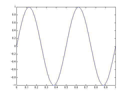
Note that this is exactly what you want to calculate and define signals. The following defines a 2
>> t = [0:.01:1];
>> s = sin(2*pi*2*t);
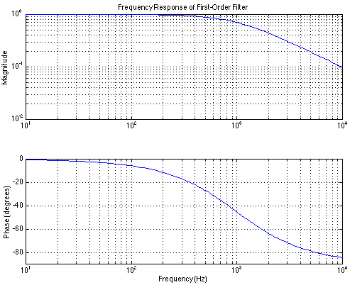
Two of the most important functions in Matlab are zeros(n,m) and ones(n,m). The first returns an nxm matrix of zeros, the second a matrix of ones. For example, the frequency response of a first-order RC circuit has the form 1/(j2 pi fR C + 1). In Matlab, this complex-valued quantity would be quite easily computed.
>>f=logspace(1,4,100);
>>H=ones(1,100)./(j*2*pi*f*R*C+1);
Note the use of ones(1,100) to form the numerator, and that using ones is not necessary when a scalar is added to a vector.
Plotting functions is very easy in Matlab. The fundamental command plot(x,y) plots the equal-length vectors on linear scales in the obvious ways. To plot our sine wave, simply type
>> plot(t,s)
and you get
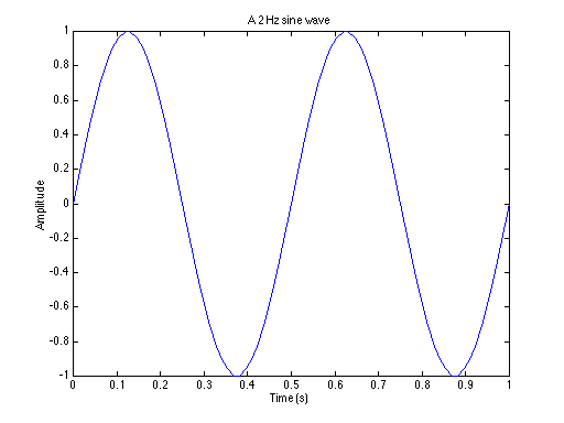
After plotting, grid places a grid on the plot, xlabel('label') and ylabel('label') place a label on the x and y axes respectively (note that ' demarcates a string in Matlab), and title('plot title') puts a title to the plot. The following commands make a more readable plot.
»xlabel('Time (s)');
»ylabel('Amplitude');
»title('A 2 Hz sine wave');
The related functions semilogx, semilogy, and loglog provide the obvious variants of logarithmic axes. Multiple plots can be placed in the same window using the subplot(n,m,k) command. Once issued, succeeding plot commands affect the kth plot measured in column order in an n x m array of plots. Usually plots are formed in some sort of sequence, with corrections to plots made once the appropriate subplot command is issued. For example,
>>subplot(2,1,1)
>>loglog(f,abs(H))
>>ylabel('Magnitude')
>>title('Frequency Response of First-Order Filter')
>>grid
>>subplot(2,1,2)
>>semilogx(f,angle(H)*180/pi)
>>grid
>>axis([10 1e4 -90 0])
>>xlabel('Frequency (Hz)')
>>ylabel('Phase (degrees)')
plots the frequency response of our first-order filter. By the way, this example contains so many commands that it would probably be better to edit them into a file (named magphase.m, for example). To form the plot, you could then just type magphase(f,H).