|
| ||
Step 1: |
Connect the
cable from the DAQ card to J3-1 on the
rightmost interface module.
| |
Step 2: |
Connect the output of the function generator to
CH1
of the scope and to
A/D input 4
(pin 46 on the bottom interface board socket connector).
| |
Step 3: |
Set the function generator to produce a 2 V p-p, 500 Hz
sine wave.
| |
Step 4: |
Download Lab5_Spectrum_Analyzer and open in Labview. Set "number of samples per channel" and "rate" to 10000. Set "averaging mode" to RMS averaging.
| |
Step 5: |
Start the instrument by selecting Run from the Operate menu, or by pressing the run button (the small arrow just below the menu bar). The instrument is divided into a display area (the large black area on the left with green lines and text) and a control area (the gray area on the right). For now, let's concentrate on the display area. It should look something like this: |
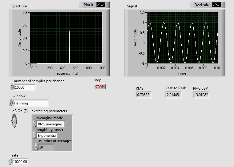
|
The top portion is the waveform display.
It should be showing a sine wave, just like the scope.
| ||
Step 6: |
There is some additional information about the signal just above
the waveform display.
The line labeled "Signal Amplitude"
gives three different measurements of the signal amplitude:
Vrms: the RMS voltage, dBV: the RMS voltage in decibels relative
to 1 V, and Vp-p: the peak-to-peak voltage.
Vary the function generator
AMPLITUDE
control and verify that these values change appropriately.
| |
Step 7: |
Disconnect the function generator.
What remains is a
noise
signal which is being generated within the rest of the system.
In this case it has both a
random
component (the grass) and a
periodic component (the 3.3 kHz signal).
| |
Step 8: |
Reconnect the function generator. Vary the frequency and observe how the spectrum display changes. |
|
| ||
Step 1: |
The Fourier series of a triangle wave has only odd harmonics,
which fall off as \(1/n^2\) (12 dB/octave).
Set the function generator to produce a triangle wave and see
if this is the case.
Are there any even harmonics?
If so, why are they there?
What happens when you vary the duty cycle?
| |
Step 2: |
The square wave also consists only of odd harmonics, but
falling off as 1/n (6 dB/octave).
Set the function generator to square wave and observe the
spectrum. Vary duty cycle.
Depending on the exact frequency
you may see a number of extraneous harmonics.
These are due to the phenomenon of
aliasing
which we will examine in Lab 6.
| |
Step 3: |
The spectrum analyzer labeled "Spectrum" displays magnitude on
and frequency on a linear scale. It is sometimes useful to view the spectrum on a semi-log or log-log plot. Stop executing the program, right-click on the spectrum display (gray area) and click on Properties->Scales. Select Log.
Adjust the amplitude if necessary to obtain a good display.
Note the hyperbolic shape of the 1/n fall off in magnitude.
| |
Step 4: |
Now get a log-log plot with magnitude in dB by changing the Y-scale to Log and setting a multiplier of 20 (under Scale Factors).
Note that the 1/f fall off is now a
"linear" 20 dB/decade slope.
| |
Step 5: |
Switch the function generator to triangle wave.
Is the slope now 40 dB/decade, as we expect?
Set the spectrum analyzer back to linear display (both magnitude
and frequency).
Note the shape of the spectrum.
| |
Step 6: |
Set the function generator to square wave.
Set the Duty Cycle to 15%.
You should now have a waveform consisting of narrow pulses.
Note the shape of the spectrum.
It should have the \(\sin(x)/x\) (sinc) shape we saw in class.
| |
Step 7: |
Set the spectrum analyzer back to dB magnitude and log frequency. Set the duty cycle to 50%. |
|
| ||
Step 1: |
Wire the following circuit:
![\includegraphics[scale=0.650000]{ckt5.1.ps}](img181.png)
This is the same circuit we used in Lab 3, so you should have
its transfer function in your lab notebook.
| |
Step 2: |
Connect the output of the function generator
to \(v_\text{in}\).
Also connect
CH1
of the scope and A/D input 4
to \(v_\text{in}\).
| |
Step 3: |
Set the function generator to produce a 50 Hz sine wave
at 1 Vrms (0 dBV).
| |
Step 4: |
Move
CH1
of the scope and A/D input 4
to \(v_\text{out}\).
| |
Step 5: |
Increase the frequency of the function generator and observe the
behavior of the spectrum display.
The tip of the peak corresponding to the fundamental of the
sine wave will trace out the magnitude of the transfer function
of our circuit.
Note that the two numbers
above the spectrum
display.
They give the
magnitude and frequency of the largest peak in the spectrum.
The "Peak Frequency" readout should correspond to the frequency
setting of the function generator.
Since the transfer function falls off as 1/f for high frequencies,
we expect the output to fall 6 dB per octave for frequencies
well above the cutoff frequency.
Check the response at 1 kHz, 2 kHz, and 4 kHz and see
how well this holds.
| |
Step 6: |
Turn off the function generator. |