| |
|

|
Step 1: |
|
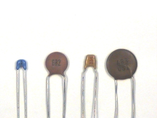
Select a 2.2 k resistor
and a .33
resistor
and a .33  F
capacitor
from your parts kit.
F
capacitor
from your parts kit.
|
Step 2: |
|
Using these components,
wire the following circuit:
![\includegraphics[scale=0.650000]{ckt7.5.ps}](img237.png)
|
Step 3: |
|
Connect the function generator to
 and the oscilloscope to
 .
.
|
Step 4: |
|
Using the technique described in the previous section,
measure the frequency response of the circuit
at the following frequencies:
20 Hz,
50 Hz,
100 Hz,
200 Hz,
500 Hz,
1 kHz,
2 kHz,
and
5 kHz.
|
Step 5: |
|
Plot the magnitude of the transfer function vs. frequency
on loglog axes and the phase on semilog axes.
|
Question 1: |
|
Using Matlab, compute and plot the expected
frequency response
for the circuit you built.
How well does this compare with what you measured?
|
Measuring a frequency response manually is time consuming and
error prone.
Since we have two more systems whose frequency response we want to
measure today, it behooves us to find a quicker way.
| |
|
|
Step 6: |
|
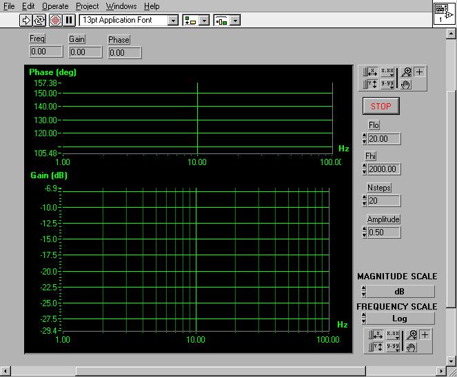
Start the program by pressing the Run button or CTRL-R.
|
Step 7: |
|
If all is well, the program will cycle through the frequencies
to be measured, displaying frequency, magnitude, and phase at each step.
However, the graph will not be drawn until all measurements are complete.
|
Step 8: |
|
When finished the program will display a plot of the magnitude and
phase of the frequency response.
How do these compare with the plots you made in Part1?
|
Question 2: |
|
From the frequency response plot, estimate  , the
frequency at which the gain has fallen to 0.707 (-3dB) of its
low frequency value.
From this value, determine the time constant.
How does this value for
, the
frequency at which the gain has fallen to 0.707 (-3dB) of its
low frequency value.
From this value, determine the time constant.
How does this value for  compare with what you measured
in Experiment 5.1?
compare with what you measured
in Experiment 5.1?
|