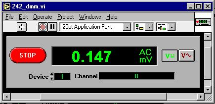
The DAQ card is interfaced to a program called "Labview" which allows us to take a signal, convert it to a sequence of samples, perform mathematical operations on them, and display the results on the PC screen. 
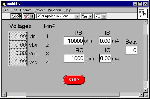
We can also generate samples of a function by computing their values and convert them to voltages to form an output signal.
Well, this is just what our lab instruments do, only with continuous functions rather than samples. This difference becomes significant when the frequency of the sampling is less than twice the bandwidth of the signal. In this lab we'll be dealing with DC and low frequency signals, so we'll quietly ignore this difference.
![]() | ||
Step 1: |
Connect the 50 pin ribbon cable from the DAQ card to P12 on the
back of the interface board.
Be sure that it goes all the way in so that the ejector latches
snap into place.
![]() | |
Step 2: |
Disconnect the BNC patch cable from the function generator
and reconnect it to the 0-6 V power supply.
![]() | |
Step 3: |
Adjust ![]() ![]() ![]() | |
Step 4: |
The input to the PC DMM is connected to A/D input 0 on the DAQ card.
This in turn is connected to pin 1 on the bottom
interface board socket connector.
Strip a piece of wire about 6 inches long to use as a probe.
Plug one end of it into pin 1 of the interface board
socket connector.
Connect the other end of it to the collector of the transistor
( | |
Step 5: |
Load the "DMM" program from the
Start menu by following the path Programs -> Labview -> 242 -> DMM.
It should look like this:
![]() ![]() | |
Step 6: |
Press the
DC Volts
button on the panel.
![]() | |
Step 7: |
Start the instrument by selecting
Run
from the
Operate
menu, or by pressing the run button (the small arrow just below
the menu bar),
or by pressing CTRL-R on the keyboard with the cursor over the panel.
The output should display the voltage of the signal (about 7 V).
![]() | |
Step 8: |
Use the PC DMM to measure the other voltages in the circuit
(![]() ![]() ![]() ![]() ![]() | |
Step 9: |
Stop the DMM program by pressing the red STOP button. |
![]() | ||
Step 1: |
Connect A/D channels 0-3 to your circuit as shown in the following
diagram.
The numbers on the connector symbols (
![]() |
![]() | ||
Step 2: |
Also add the 1 nF capacitor shown in the diagram.
This capacitor is a bit of magic to avoid anomolous behavior.
![]() | |
Step 3: |
Load the "CE Voltmeter" program from the Start menu by following the path Programs -> Labview -> 242 -> CE Voltmeter. It should look like this: |
![]() | ||
Step 4: |
Start the program by pressing the Run button or CTRL-R.
![]() | |
Step 5: |
If necessary, adjust ![]() ![]() ![]() | |
Step 6: |
The program also calculates the base and collector currents
and beta.
Do these agree with your earlier values?
![]() | |
Step 7: |
Repeat the transfer characteristic measurements you made in
Part 2 of
Experiment 3.1.
Plot ![]() ![]() ![]() | |
Step 8: |
Stop the program by pressing the red STOP button. |
![]() | ||
Step 1: |
Disconnect ![]() |
![]() | ||
Step 2: |
Load the "CE Curve" program from the
Start menu by following the path Programs -> Labview -> 242 -> CE Curve.
![]() | |
Step 3: |
Start the program by pressing the Run button or CTRL-R.
The value displayed for "Vin" on the panel should
begin to increase in 0.1 V steps.
You should be able to verify this from the scope.
The program also displays the corresponding value of "Vout".
![]() | |
Step 4: |
After 25 steps, the program will display the plot of ![]() ![]() ![]() | |
Step 5: |
Close the various PC Instruments by clicking the "X" box in the upper right hand corner of each window. Answer "No" if the question "Save changes to xxx.vi" appears. Disconnect the ribbon cable from the interface board by using the ejector levers. Do not try to remove it by pulling on the cable. |