ELEC 243 Lab
Experiment 2.1
The Oscilloscope and Function Generator
Equipment
So far we've measured only constant (or nearly constant)
voltages and currents.
Although these are important,
as signals they are fairly boring.
A much more interesting (and information rich) class of
signals are
time varying
voltages and currents.
For a slowly time varying signal, we could just
write down the values as they change (as we did in
plotting the light bulb I-V curve), but for
most time varying signals we need something
a bit faster.
That faster something is the
oscilloscope
(from the Latin
oscillare
to swing + Greek
skopion
to look at).
In order to measure time varying signals, we need a source of time varying signals.
The DC power supply is our source of constant voltages,
the
function generator
(from the English
function
a mathematical relation +
generator
a machine that produces electricity)
is our source for that class of time varying signals known as
periodic signals.
Part 1: Viewing Signals with the Oscilloscope
Making a measurement with the Oscilloscope consists of two
phases: (1) getting it to display anything at all, (2) getting it
to display what you want.
If any one of several important controls is not properly set, no display at
all will appear, so the first order of business is to get all of
these controls into a reasonable state.
We have two different types of oscilloscopes: the Iwatsu SS-5702
and the Leader LS 1020.
These are largely similar, but where there are differences,
the control or operation for the Leader will be given in parentheses.
| |
|

|
Step 1: |
|
Set the oscilloscope controls as follows:
- Power: ON
- Intensity: Mid scale
- V Mode: CH 1
- Vertical Position (both knobs): Mid scale
- Volts/Div (both knobs): 2V
- Variable Volts/Div (both knobs): Fully clockwise
- AC-GND-DC (both switches): DC
- Polarity: Normal (CH 2 Position IN)
- Horizontal Position: Mid scale
- Time/Div: 1ms
- Variable Time/Div (Time Variable): Fully clockwise
- Sweep Mode: Auto (Holdoff button pressed in)
- Trigger Source: CH 1
- Trigger Level: zero
- Trigger Coupling: AC
If everything is in order, you should see a blue-green horizontal
line through the middle of the screen.
|
Step 2: |
|
Set up the function generator to produce a 1kHz sine wave:
- Power: ON (can't be turned off)
- Duty: Pressed in and fully counterclockwise
- Offset: Pressed in
- Ampl: Pressed in and mid scale
- Range: 1K
- Function: Sine
- Frequency: 1.0
|
Step 3: |
|
Connect the function generator's
main
OUTPUT
( )
to the oscilloscope's
CH 1
input.
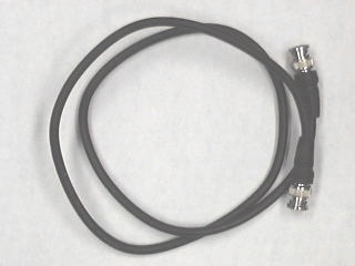
The easiest way to do this is to connect one end of a
BNC patch cord
to the function generator and the other to the oscilloscope.
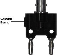
This connects the generator's ground and signal terminals
to the scope's ground and terminals.
If all has gone well, you should see about 10 cycles of
a sine wave.
)
to the oscilloscope's
CH 1
input.
The easiest way to do this is to connect one end of a
BNC patch cord
to the function generator and the other to the oscilloscope.
This connects the generator's ground and signal terminals
to the scope's ground and terminals.
If all has gone well, you should see about 10 cycles of
a sine wave.
|
Step 4: |
|
Now examine the effect of each control.
Move the display with the positioning controls.
Change the timebase to see what effect is produced.
Pull the red
X1-X5
switch in the middle of the timebase's position knob
(pull out the
H POSITION
knob).
What does this do?
What is the effect of changing the slope control from
"+" to "-"?
Change the vertical amplifier settings to see the effect that they have.
If you turn the red knobs in the center of the vertical amplifier
adjustment, you place the oscilloscope in an uncalibrated mode.
Do this and see what happens.
|
Step 5: |
|
Examine the various waveforms produced by the function generator.
Examine the effects of the
DUTY
and
OFFSET
controls
(must be pulled out to function).
Before going on, be certain that you are comfortable with the
oscilloscope and function generator.
If you are having problems, ask your labbie for help.
|
Part 2: Quantitative Measurements with the Oscilloscope
In addition to allowing us to view the "shape" of a signal,
the oscilloscope can also measure voltage, amplitude,
time intervals, and frequency.