![\includegraphics[scale=0.500000]{flashlight2.ps}](img227.png)
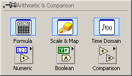
If all we could with Labview was to make computer based copies of our conventional instruments, it would be of limited use. What makes Labview so valuable is that it is programmable. By changing the program a single box (the Lab PC) can perform the functions of a large collection of instruments, both conventional and unconventional. Some of the instruments in this collection are ready-made, for example those in the program menu entries for this course and the other ELEC lab courses.
Perhaps the greatest advantage of Labview however, is that it is user programmable: if no instrument is available which meets your requirements, you can modify an existing one or create an entirely new one.
Our goal for this Experiment will be to measure the resistance of the thermister and display the result directly as a temperature reading. Since the DAQ card can only measure voltage, our first step is to convert the resistance to a measureable voltage, but we already know how to do this from Part 5 of Experiment 1.1. As a reminder, here's the circuit we used.
We need to make a few changes to the above circuit. Obviously we need to replace the light bulb with the thermistor. Since the thermistor has a much higher resistance, we should also replace the 10Ω resistor with one closer to the nominal resistance of the thermistor, in this case 10kΩ. In addition, since our goal is to measure temperature we will need to convert the measured resistance into a displayed temperature reading.
|
| |||
Step 1: |
Use a BNC-Banana adapter and a BNC patch cable
to connect the 0-6 V power supply to J1-3,
as you did in Part 1 of Experiment 3.1.
| ||
Step 2: |
Wire the following circuit
(![\includegraphics[scale=0.500000]{ckt3.3.4.ps}](img228.png)
| ||
Step 3: |
Using your DMM, set the 0-6 V supply output
(
| ||
Step 4: |
Load and start the DMM-Scope Labview program
that you used in Part 2 of Experiment 3.1.
Set the
AD Channel
knob to 5
and verify that | ||
Step 5: |
Since we are going to build
a VI from scratch,
we will start with a new, blank VI.
Stop the DMM-Scope VI and select
"New VI"
from the "File" menu.
A pair of windows should appear.
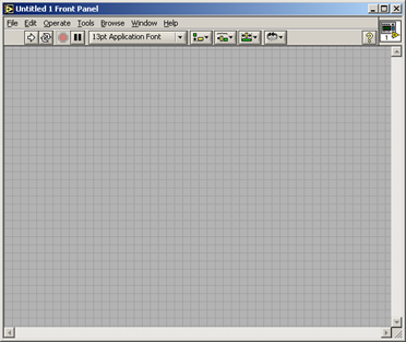
The one on top will be a blank Front Panel window:
| ||
Step 6: |
Our first effort will be the simplest
possible VI that will actually do something:
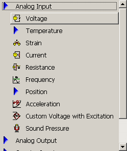
we will measure Right click over the panel window. You will get the Controls popup: 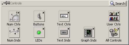
| ||
Step 7: |
A pair of boxes with an open hand cursor will
appear on the front panel.


Type "VT" and left click the check-mark box at the
upper left of the window (

| ||
Step 8: |
Now we need something for the indicator to display.
Click on the Block Diagram window to bring it to the top.
This may also bring up the Functions palette.
If so, move it out of the way or click the close box.
Note that placing the indicator on the front panel
has also placed a block on the block diagram.

| ||
Step 9: |
If you closed the Functions palette in the previous
step, right click to bring it up.
| ||
Step 10: |
Wait patiently.
You may briefly see a dialog labeled "Initializing".
After a second or two the "Create New .." wizard will appear.
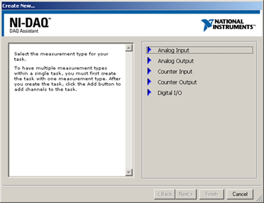
| ||
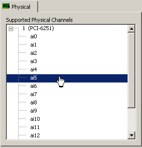
Step 11: |
From the list of Supported Physical Channels
that appears, select "ai5",
| ||
Step 12: |
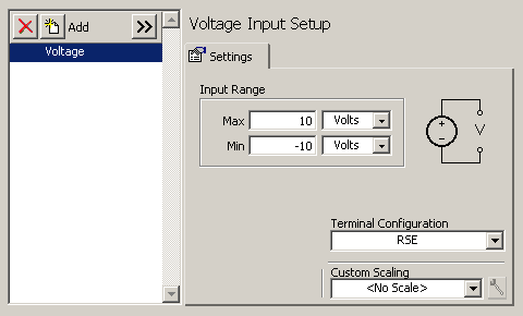
After another brief wait, the "DAQ Assistant" dialog appears.
In the "Input Range" block set "Max" to 10 Volts
and "Min" to -10 Volts.
Set the "Terminal Configuration" field to "RSE".
The upper half of the panel should look like this when you are done.
| ||
Step 13: |
Things will click and whir for several seconds.
When it's all over, the "DAQ Assistant" box will have
expanded, and should have a white band with the word
"data" in it.
| ||
Step 14: |
We're almost done. All that remains is to connect the
source (A/D converter block) to the destination
(numeric indicator block). This process is called
wiring.
Place the cursor over the small black triangle in the "data" field of the DAQ Assistant block. It should change into an icon representing a small spool of wire. Left click once and move the cursor to the small white triangle in the center of the left edge of the numeric indicator icon and left click once more. That completes our first Labview program. It should look something like this: 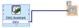
| ||
Step 15: |
Let's try it out.
Click on the Front Panel window to bring it to the top.
Run the VI by clicking on the Run arrow
or by typing Ctrl-R.
The
VT
nemeric indicator
should display the voltage across | ||
Step 16: |
It's always a good idea to save your work from time to time,
and since we currently have a working VI, this would be a
good time.
Select
Save As...
from the
File
menu.
Set the
Save in:
field to an appropriate directory
(e.g. the desktop, your network home directory, or
your local
Group nn
folder).
If "Untitled.vi" seems like an inadequate name for such a momentous work, think of a more descriptive one (e.g. "lab3.vi") and enter it into the File name field. When everything is in order, press the Save button. |
There are two ways we could formulate this calculation.
We could do it in two steps, first computing
![]() ,
then using Ohm's Law to get
,
then using Ohm's Law to get
![]() .
Alternaltely, we could treat the circuit as a voltage
divider, which with a little manipulation gives
.
Alternaltely, we could treat the circuit as a voltage
divider, which with a little manipulation gives
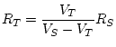
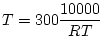
Because we will be interested in ![]() in a subsequent Experiment, we will use the first approach.
in a subsequent Experiment, we will use the first approach.
|
| ||
Step 1: |
On the front panel, create a new numeric indicator
and label it
IT.
You can place it anywhere, but a convenient location
would be near the existing indicator.
| |
Step 2: |
In order to compute the current we will have to do
some arithmetic on the
| |
Step 3: |
Let's start with the subtraction.
Move the cursor over the symbol labeled
Subtract
and left click.
Position the icon below the existing components on
the diagram and left click to put it down.
Note that while the cursor is over the symbol there
are three small circles near the vertices of the triangle.

| |
Step 4: |
Repeat the above process, but select the
Divide
symbol.
Place it slightly to the right and a little lower
than the subtract icon.
| |
Step 5: |
Now let's do the constants, starting with 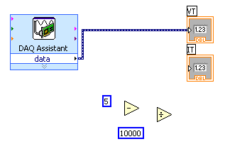
| |
Step 6: |
All that remains is to make the connections.
We already know how to do this from the previous Part:
place the cursor over a connection point, wait for it
to turn into a spool of wire, click, move to the other
terminal, and click again.
A couple of things to note:
1. The position of the terminals on the arithmetic blocks corresponds to the conventions of grade school arithmetic. For subtract the minuend is on top and the subtrahend is on the botton. For divide the dividend is on top and the divisor on the botton. 2. To connect to an existing wire (in this case the one between the A/D converter block and the VT display block), move the cursor near, but not directly on, the wire. If you place the cursor on the wire it will turn into an arrow, indicating that you can select the wire. When you're done it should look something like this: 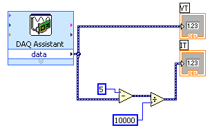
| |
Step 7: |
Let's test what we have so far.
Go to the front panel and click on the
Run
button.
If all is well, | |
Step 8: |
Now that we have found the current in the thermistor,
finding the resistance is easy: just divide 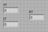
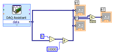
| |
Step 9: |
Test the VI by clicking Run from the front panel. The RT indicator should display a value close to 10000. |
|
| ||
Step 1: |
Based on the information in the
thermistor data sheet,
derive a formula which gives the temperature
(your choice of K, °C, or °F)
in terms of the resistance of the thermistor.
| |
Question 3: |
After convincing yourself that your formula is correct,
summarize your derivation in a form that will convince
your labbie.
| |
Step 2: |
If your formula is correct, it should be somewhat more complicated
than the one required to convert In the Block Diagram window, right click to bring up the Functions palette. Move the cursor to the All Functions button to bring up the Functions palette. 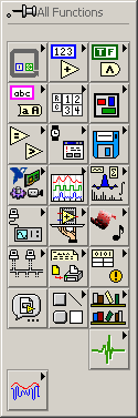


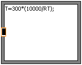
The formula node is a variable sized block, so it is instantiated by clicking on the desired location of the upper right corner and dragging to create the desired size. Move the cursor to a convenient spot on the block diagram, preferably near the RT indicator icon, then click, drag, and release to create the formula node. It should look like this: 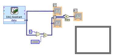
| |
Useful Tip |
If you want to find out more about the components in the block
diagram, you can turn on the
Context Help
feature:
select
Show Context Help
from the
Help
menu.
When context help is turned on, a window
(labeled
Context Help)
appears in the upper right corner of the screen.
When the cursor is moved over any component in the
block diagram,
a brief description and a link to additional information
appears.
Since the context help window insists on always being on top,
it can be a nuisance when you aren't using it.
To make it go away until you need it again, click the close button.
| |
Step 3: |
A new formula node is not of much use.
It has no formula, and it has no inputs or outputs.
Let's start with the formula.
As an example, we'll use
 .
(If you got this formula, you should check your derivation,
as it is not correct.)
Since we can't type subscripts in labview, we will use
.
(If you got this formula, you should check your derivation,
as it is not correct.)
Since we can't type subscripts in labview, we will use
| |
Step 4: |
At this point you may have noticed a change in the appearance of the
toolbar: the run button has changed from a white arrow to a
gray broken arrow
(
 ).
This means that there is an error in the
block diagram and the VI won't run.
To find out what the error is, click on the broken arrow button.
).
This means that there is an error in the
block diagram and the VI won't run.
To find out what the error is, click on the broken arrow button.
If you do this you should find that the problem is an
undefined variable.
Actually, there are two: | |
Step 5: |
Place the cursor somewhere on the left-hand border of the
formula node and right-click. Select
Add Input
from the popup menu.
This should create a small rectangular box in the border.
| |
Step 6: |
The arrow is still broken, but now
the error message complains of an "unwired input."
Let's try to fix that:
connect the input
(RT) to the wire between the division block and the
numeric indicator which displays the value of | |
Data Types: |
Like many programming languages (e.g. C) Labview
maintains the notion of
data types.
Labview's data types
include familiar ones such as integer, floating point,
boolean, and string,
as well as a number of unfamiliar ones
(which we will try to avoid for the time being).
Labview denotes data type by the color of the wire
which carries it: integer wires are blue, floating point
wires are orange, boolean wires are green, and
strings are pink.
Labview also supports collection types, such as arrays
and structures.
Scalars are denoted by thin solid lines, arrays by
thick solid lines, and other collections by various
patterned lines.
The wide dark blue lines with internal dashes are
a composite data type called
dynamic data.
Dynamic data contains a lot of information in addition
to the value of the sample,
for example, the time at which the sample was taken,
whether any errors were made in previous handling of the
sample, etc.
Dynamic data usually makes life easer for us
by bundling ancillary information along with a signal
so we don't have to be concerend about carrying it around
separately,
but at the moment it's causing problems.
While most blocks (e.g. subtract, divide, numeric indicator)
can accept any appropriate data type, including dynamic,
others are more picky about what they will take.
For example, the formula node expects ordinary, pure numeric data
and doesn't know what to do with the additional stuff contained
in dynamic data.
We can fix this by converting the dynamic data to
scalar data.
| |
Step 7: |
Remove the offending broken wire.
To do this, place the cursor directly over the wire,
so that it turns into an arrow, and double click.
Press the
Delete
key.
| |
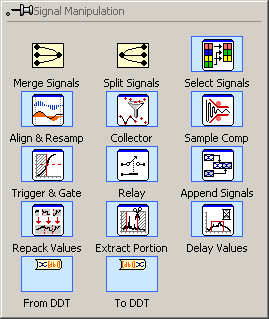
Step 8: |
Right click to bring up the
Functions
palette.
Place the cursor over the
Sig Manip
button to bring up the
Signal Manipulation
palette.
| |
Step 9: |
When you place the
From DDT
block, a dialog box labeled "Convert from Dynamic Data"
will appear.

| |
Step 10: |
Wire the output of the
From DDT
block to the
RT
terminal of the formula node.
Connect the input of the
From DDT
block
to the wire between the division block and the
RT
numeric indicator.
The arrow should now be unbroken.
| |
Step 11: |
All that remains is to display the value of temperature
that we have gone to so much trouble to calculate.
Place another numeric indicator at an appropriate location
on the front panel and label it
T.
Return to the block diagram, position the new indicator
icon just to the right of the
T
terminal of the formula node,
and wire them together.
Here's what you should have:
| |
Step 12: |
Return to the front panel and press the run button. If all is well, the T indicator will display the current temperature. |
|
| ||
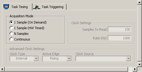
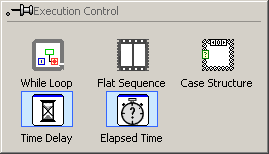
Step 1: |
Right click in the block diagram to bring up the
Functions
palette.
Move the cursor to the
Exec Ctrl
button to bring up the
Execution Control
palette.

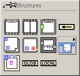
This is a variable sized block, like the formula node, and we want it to enclose everything we currently have in our VI. Bring the cursor into the block diagram window and click above and to the left of all blocks, then drag until everything is enclosed and release.
Note the green-bordered block labeled
stop
in the lower right corner of the while loop.
This is a free accessory that allows us to stop the
loop, which would otherwise run forever.
This block is an example of a
control.
A control is the dual of an indicator,
i.e. it provides input from the front panel
to the block diagram.
Go to the front panel and notice that there is a
new object, a button labeled
STOP.
Pressing this button causes the associated icon
to output a
True value
(when the button is not pressed, the output is
False).
| |
Step 2: |
From the front panel, press the
Run
button.
The indicators should now display continuously updated
values.
To convince yourself that these aren't random,
grab the body of the thermistor between your
thumb and forefinger, being careful not to
touch the leads.
The displayed temperature should increase.
When it stabilizes, or you get tired of pinching
the thermistor, press the
STOP
button.
| |
Step 3: |
The updating of the display, while certainly continuous,
might also be described as frantic.
This is because new samples are being taken and displayed
as fast as the A/D converter is able to take them
(1,250,000 samples/second),
which is much faster than any phenomenon we might bring
into the lab is capable of changing its temperature.
The net result is wasted processor power and a blurry
display which is difficult to read.
There are a number of ways in which we can set the sampling rate to a more reasonable value. We will utilize one which requires minimal change to what we have already constructed. Return to the block diagram and again bring up the Execution Control palette. This time select the Time Delay block 
| |
Step 4: |
Return to the front panel and click
Run.
The display should now update at a more leisurely rate.
| |
Step 5: |
Be sure to include a printout of your block diagram in
your lab writeup.
You can do this with
Print Window ...
from the
File
menu.
| |
Step 6: |
Save your work in a persistant location (not the desktop). We will make further enhancements next week. |
 ).
The indicator is now ready for use.
).
The indicator is now ready for use.