As we saw in the previous experiment, the op-amp isn't
very useful in an "open-loop" configuration
(i.e. without feedback).
The most common configuration for op-amp circuits is the
inverting amplifier
where the output is an amplified and inverted version of the
input
(i.e. ![]() is negative).
From this starting point we can create a number of different
input-output relationships, including sum, difference, and
non-inverted gain.
is negative).
From this starting point we can create a number of different
input-output relationships, including sum, difference, and
non-inverted gain.
|
| ||
Step 1: |
Wire the following circuit using 10 k![\includegraphics[scale=0.650000]{../241/inv_opamp.ps}](img234.png)
Fig. 5.1: Inverting Amplifier | |
Step 2: |
Set the function generator to produce a 1 V p-p, 100 Hz
sine wave.
Measure the voltage gain,
In particular, note that the output is inverted with respect
to the input.
| |
Step 3: |
Replace | |
Step 4: |
Increase the input amplitude until output clipping occurs.
What is the clipping level?
Is it the same as in Exp. 5.1?
| |
Step 5: |
Reduce the input amplitude till the output is 20 V p-p.
| |
Step 6: |
Increase the frequency until
the output amplitude drops to 10 V p-p.
You should see a triangular output waveform.
This is because there is a limit to the maximum rate at which the
output voltage can change, called the
slew rate.
Set the input to triangle and square wave and see how
the output changes.
| |
Step 7: |
Reset the function generator for a 100 Hz sine wave and reduce the amplitude to produce a 1 V p-p output from the op amp. (You may need to use the 20 dB attenuator on the function generator.) Again increase the frequency until the output is 0.7 V p-p. Observe that the output is still sinusoidal. This is the actual cutoff frequency or bandwidth of the amplifier. |
The inverting amplifier is the basis of many different op-amp circuits. Once you understand it you can analyze and design a large variety of functional elements. And once you know how to construct it you should be able to construct any op-amp circuit with a minimum of assistance. So from now on, we will abandon the detailed, step-by-step procedures, telling you exactly which pin to connect to which other pin, and allow more freedom for you to determine your own procedure. The instructions will simply tell you what needs to be done, you get to decide how to do it.
The inverting amplifier configuration we used makes this very easy to do, just add another resistor to the inverting (-) input of the op amp:
![\includegraphics[scale=0.650000]{opamps/summer.ps}](img235.png)
|
| ||
Design: |
Rather than just add two arbitrary signals together and
watch the result on the oscilloscope, let's do something
a bit more entertaining: add two signals together and
listen to them.
From our observations in Part 1 of Experiment 2.2
and Part 1 of this Experiment, we would expect to have
trouble driving the loudspeaker with the output of the
op-amp.
Fortunately, we have a more suitable acoustic
output transducer: the earpiece of the telephone
handset.
The telephone earpiece is also very easy to connect to:
just plug it into J1-7 and wire to the appropriate pins on
the interface module connector strip.
Notice that, unlike the microphone,
neither of the two earpiece terminals is automatically grounded.
Be sure to ground one and connect the other to
For our two inputs, we will use the function generator
for | |
Construction: |
Start by building the circuit
shown in Fig. 5.2
using the component values you determined in the
previous step.
Connect | |
Testing: |
When the circuit is completed,
speak into the
microphone at a normal speaking level
and verify that the output | |
Observations: |
Set the function generator to produce a 440 Hz sine wave. Adjust the amplitude to produce a comfortable listening level in the handset earpiece. While listening to the earpiece and watching the oscilloscope, sing, hum, or whistle the note A (hint: 440 Hz). Describe what happens, both aurally and visually when you are in tune and when you are slightly out of tune with the function generator. If the range of your voice does not encompass A440, try tuning the function generator down an octave to 220 Hz. |
![\includegraphics[scale=0.500000]{ckt7.1.1.ps}](img236.png)
This is an example of the basic
non-inverting
op-amp configuration.
A simple analysis shows that
![]() (with no minus sign).
This circuit has a couple of useful characteristics.
Most obvious is that it doesn't invert.
Another is that the input impedance is extremely high.
One potential disadvantage is that the minimum value of
gain is unity.
(with no minus sign).
This circuit has a couple of useful characteristics.
Most obvious is that it doesn't invert.
Another is that the input impedance is extremely high.
One potential disadvantage is that the minimum value of
gain is unity.
|
| ||
Construction: |
Using a 741 op amp,
wire the circuit of Fig. 5.3.
Let | |
Testing: |
Connect a 1 V p-p 1 kHz sine wave
(or any other waveform of similar amplitude and frequency)
to | |
Observations: |
What is the actual gain?
Is it in fact non-inverting?
What happens with nothing (i.e. an open circuit)
connected to |
![\includegraphics[scale=0.500000]{opamps/diff2.ps}](img237.png)
For arbitrary values of the resistors, we get
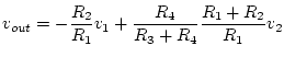 which doesn't seem very useful.
However, if we let
which doesn't seem very useful.
However, if we let ![]() and
and ![]() , then we have
, then we have
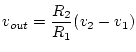 i.e. a
difference amplifier.
i.e. a
difference amplifier.
|
| ||
Construction: |
Wire the above circuit, using 10 kΩ for all four resistors.
| |
Testing: |
Using the function generator for |