Although we usually think of a fan as a device which produces flow, since it has to drive that flow through the constricted air paths inside the equipment it is cooling, our fan must also be capable of producing pressure, i.e. it is also a pump.
Since we now have a device that can produce pressure and a device that can measure pressure, we can combine them to produce a system that regulates pressure i.e. a control system.
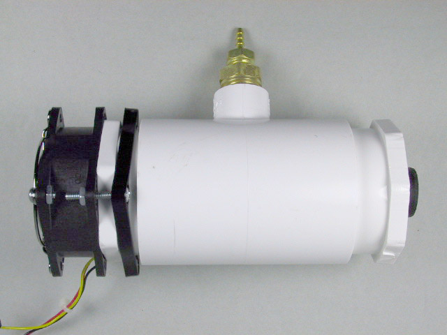
In order to build up a pressure we need to confine the output of the fan to a reasonably small volume. To facilitate this we have assembled a pressure control assembly from space-age plastic components. The fan assembly from the previous Experiment conveniently slips into one end of the structure, and the vinyl hose from the pressure sensor fits onto the barbed fitting in the center.
|
| ||
Wiring: |
If the connections from Experiments 8.1 and 8.2
are intact, there's no more wiring to do.
| |
Assembly: |
Start the VI.
If necessary, reset the
Offset
value so that the
Pressure
reads zero when nothing is moving.
Slip the fan assembly into the open end of the tee fitting.
It should fit snugly, if not wrap a layer of tape around it.
Push the end of the vinyl hose
(whose other end should be connected to the pressure port
of the pressure sensor)
onto the barb fitting in the center of the tee.
The remaining branch of the tee should be sealed with a rubber stopper.
The assembly will vibrate when running,
so be sure that it is placed so that it will not fall off
of the bench, or else have your lab partner hold it.
| |
Testing: |
Start the VI and turn on the power.
Increase the setting of the
Motor
control slider.
As the fan begins to turn, you should get a positive
pressure reading, which should increase to a value of
about 0.13-0.15 kPa with the control at maximum.
If the pressure is negative,
take appropriate action to reverse the sign.
The easiest fix is to move the tubing to the
other port of the pressure sensor.
| |
Characterization: |
Measure and plot pressure vs. motor drive at an appropriate number of points. Repeat the characterization with the rubber stopper removed. |
This is an example of manual control, similar to the way you control the speed of your car when not using the cruise control. The changing of the set point corresponds to moving between different speed zones and the insertion and removal of the stopper is a form of disturbance. Disturbances are uncontrolled external inputs (e.g. a wind gust) or changes in system parameters (e.g. a hill) which necessitate an adjustment to the controlling input in order to maintain the desired output.
Although a certain amount of enjoyment results from controlling the speed of a car, controlling the speed of the fan gets old in a hurry. This is clearly a process which should be automated. There are two approaches we could try: (a) find the correct value of the controlling input and maintain that value until something changes (as we did with manual control), or (b) switch between two speeds, full on or off, in such a way as to keep the the controlled variable acceptable limits. We'll try approach (b) first, since it's easier.
|
| ||
Setup: |
Select the
On-Off
tab of the tab control panel.
| |
Testing: |
Start the VI.
The pressure should oscillate in a small band
around the set point.
| |
Observations: |
Adjust the hysteresis, change the set point, insert and remove the stopper. Observe how the system responds. |
In proportional control, the value of the error
is multiplied by a constant (![]() ) and used as the
input to the driving amplifier.
Since this involves feeding a sample of the output
back into the input of the system, it is called
feedback control.
A little thought shows that if a non-zero input
is required in order to have a non-zero output
(as is in the case with our pressure control system),
then the error can never be driven completely to zero
(since the input is a multiple of the error).
) and used as the
input to the driving amplifier.
Since this involves feeding a sample of the output
back into the input of the system, it is called
feedback control.
A little thought shows that if a non-zero input
is required in order to have a non-zero output
(as is in the case with our pressure control system),
then the error can never be driven completely to zero
(since the input is a multiple of the error).
However, if we
integrate
the error before feeding it back into the input, then
it is possible to have a zero steady-state error.
A controller which does this is called an
integral controller.
As with the proportional controller, there is a parameter
![]() , called the
integrator gain,
which adjusts the amount of integrated error fed back
to the input.
, called the
integrator gain,
which adjusts the amount of integrated error fed back
to the input.
An integral controller can achieve zero error, but is sluggish. A proportional controller can respond quickly, but can't achieve zero error. By combining the two, we get a proportional-integral (PI) controller.
![\includegraphics[scale=0.500000]{ckt8.3.2.ps}](img255.png)
In the diagram ![]() is the Laplace Transform notation for
integration, so
is the Laplace Transform notation for
integration, so ![]() represents
represents
![]() .
.
|
| ||
Setup: |
Select the
Proportional
tab of the tab control panel.
| |
Testing: |
Start the VI.
The pressure should settle to a value
very close to the set point.
| |
Characterization: |
With the default values of
Turn the integrator
off
and observe how effective proportional control alone is.
Try various values of
Turn the integrator back on
and try various combinations of |