![\includegraphics[scale=0.500000]{ckt7.3.1.ps}](img266.png)
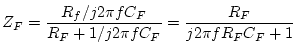
In the previous Experiment we converted a voltage divider, whose attenuation is independent of frequency, to a filter by replacing one of the resistors with a capacitor. If we substitute a capacitor for a resistor in the inverting op-amp circuit, we can effect a similar transformation from a constant gain amplifier to a filter where gain depends on frequency. We can analyze the response to sinusoidal signals by representing the input and feedback elements as impedances:
In this Experiment we will explore the result of
using various components and combinations of components for
![]() and
and ![]() .
Since we will be making a number of frequency response plots
we will want to use the
Labview "Transfer Function"
program that we used in Experiment 8.1.
Here is a diagram of the required connections:
.
Since we will be making a number of frequency response plots
we will want to use the
Labview "Transfer Function"
program that we used in Experiment 8.1.
Here is a diagram of the required connections:
![\includegraphics[scale=0.500000]{ckt7.3.7.ps}](img267.png)
 .
Since
.
Since ![\includegraphics[scale=0.500000]{ckt7.3.8.ps}](img268.png)
|
| ||
Construction: |
Wire the circuit of Fig. 7.3 using
| |
Testing: |
Verify that the circuit works using the function generator
as an input.
| |
Characterization: |
Using the Labview transfer function VI, measure and record the frequency response between 20 Hz and 2 kHz. |
By placing the capacitor in the input network we can make a high-pass filter:
![\includegraphics[scale=0.500000]{ckt7.3.2.ps}](img269.png)
|
| ||
Construction: |
Wire the circuit of Fig. 7.7 using
| |
Testing: |
Optional. If you're confident of your wiring,
proceed to the next step,
otherwise test with function generator and oscilloscope.
| |
Characterization: |
Using the Labview transfer function VI, measure and record the frequency response between 20 Hz and 2 kHz. |
We could combine the high-pass input network with the low-pass feedback network to make a band-pass filter.
![\includegraphics[scale=0.500000]{ckt7.3.3.ps}](img270.png)
![\includegraphics[scale=0.500000]{ckt7.3.4.ps}](img271.png)
![\includegraphics[scale=0.500000]{ckt7.3.5.ps}](img272.png)
|
| ||
Construction: |
Wire the circuit shown in Fig. 7.7
using
| |
Testing: |
Optional again.
| |
Characterization: |
Measure and record the frequency response
between 60 Hz and 6 kHz.
Because of the sharpness of the peak in the
frequency response, you should use a larger number of steps,
say 40.
| |
Question 2: |
Analyze the three circuits used in this Experiment and compare the calculated frequency response with that which was observed. For the low-pass and high-pass filters, compare your results with the corresponding circuits from Experiment 8.1. |