![\includegraphics[scale=0.500000]{ckt7.1.6.ps}](img277.png)
The analog filters we looked at last week have the advantage of simplicity and low cost, but they also have relatively low performance. Much higher performance analog filters are possible, but they are correspondingly more complex, and difficult to construct. Digital filters are capable of much higher performance, and since we already have Labview up and running, most of the construction is already done. The one caveat with digital filters is that we have to be careful to avoid aliasing.
|
| ||
Construction: |
Add a 1 nF capacitor to your photodiode amplifier
as shown in the circuit above.
Remove the 4.7 kΩ resistor and .033 µF
capacitor used in last week's filter
and connect
| |
Testing |
Start the "Spectrum" VI and verify that things still behave the same as they did at the end of last week's Lab. |
Let's start by building a VI that simply copies a continuous input stream to a continuous output stream, i.e. a Labview wire. We can do this by putting a A/D converter block and a D/A converter block inside a while loop and connecting the A/D output to the D/A input.
|
| ||||||||||||||||||||
Construction: |
Start Labview and build a new VI with the following block diagram:
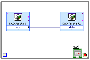
For the output set Analog Output and Voltage, then
Also check the "Use timing from waveform data" box.
| |||||||||||||||||||
Setup: |
We are going to apply our Labview filters to the photodiode
amplifier output.
Since we now have a built-in anti-aliasing filter
we can connect the
photodiode amplifier directly to the Labview A/D input,
as shown in the following diagram.
![\includegraphics[scale=0.500000]{ckt7.1.7.ps}](img278.png)
We will assess the results of our filtering by a number of
means, including watching and listening,
so connect the Labview D/A output to
CH2
of the oscilloscope and to
the handset earpiece.
As inputs, plug in the microphone and connect the
function generator to | |||||||||||||||||||
Testing: |
Turn everything on and start the VI.
Speak into the microphone and play with the function generator.
You should be able to hear the sounds in the earpiece
and see them on the oscilloscope,
just as you did last week in Part 5 of Experiment 6.3.
When everything is working correctly, save your VI as "wire.vi". |
|
| ||
Construction: |
Remove the wire between the A/D DAQ Assistant block
and the D/A block.
Place a
Filter
block (located in the
Analysis
palette of the
Functions
popup)
between the two.
In the
Configure Filter
dialog, accept the defaults (for now).
Connect the D/A
data
output to the filter
Signal
input and connect the
Filtered Signal
output to the A/D
datainput.
If your blocks are very close together, Labview may try to automatically make connections for you. In particular, it may connect the error out of one block to the error in of the adjacent block, using a pink wire. If it makes automatic connections that you don't approve of, simply remove them. When you get done, it should look like this: 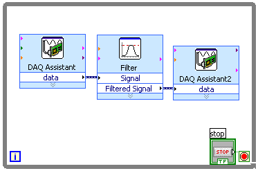
| |
Testing: |
Perform the same tests as in the previous Part. Because of the fairly aggressive filtering the sound will be rather muffled. |
|
| ||
Construction: |
The first thing we need is a switch.
Go to the front panel and select an appropriate
one from the
Buttons and Switches
palette (press the
Buttons
button on the
Controls
popup).
Change the label to something meaningful like "Filter On."
Return to the block diagram and move the new icon (a green box with a picture of your chosen switch in it) to a position below the filter block. From the Functions popup select Comparison then Select. Place the resulting icon to the right of the switch icon. The select block has three inputs and one output. The middle input is the selector: connect it to the switch. (The resulting green wire indicates a boolean signal.) Connect the output to the data input of the D/A block. Connect the upper input to the filter output and the lower input to the A/D output. Here's what you should have: 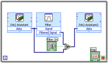
| |
Testing: |
Fire everything up and listen to the earpiece while flipping
the filter on/off switch back and forth.
You should be able to hear the difference between filtered and unfiltered.
| |
Observations: |
With the default values for the filter block
(100 Hz lowpass) the
noise at the output of the filter
will be less than the noise at the input, but so will the signal.
Have your lab partner speak into the microphone and try various
combinations of filter in vs. filter out,
under-shelf florescent light on vs. off, etc.
Is the speech intelligible with the filter turned on?
We can reduce the amount of damage to the speech signal by increasing the bandwidth of the filter. To do this, stop the VI, double click on the filter block, enter a new value for Cutoff Frequency, and click OK. Try several different values and report on the results. |
|
| ||
Setup: |
Load the "Filters" VI from the ELEC 243 Start menu.
It has the same connections as the VIs in previous Parts,
so no rewiring is necessary.
The under-shelf florescent lamp should still be on to
provide a source of noise to be filtered.
| |
Operation: |
As promised, this VI has a number of new goodies.
Most prominant are the four graph displays.
The top two show the input waveform and spectrum
and the bottom two show the filtered output.
Underneath the waveform displays is a slider to adjust
the time scale. The
Full Range
button overrides the slider and displays the entire signal.
Similarly the slider and button under the spectrum displays
control the displayed frequency range.
The selection of filter type and adjustment of filter parameters are under control of the tab control in the center left of the front panel. 
Finally there are two numeric indicators which show the
RMS value of the input and output signals.
These can be used in computing SNR.
| |
Inside the VI: |
Open the block diagram by selecting
Show Block Diagram
from the
Window
menu.
The overall structure is similar to the VI from the previous Part,
but includes displays similar to those of the
Spectrum
VI.
One important addition is that the various filters are selected
by a case block rather than a selector block.
The case block is the
equivalent of a case statement in conventional
programming languages.
Only the functions in the selected page are executed, the contents of
the other pages are ignored.
The selection is determined by the value on the selector input,
which in this case is connected to the tab control icon.
To view the different pages, place the cursor over the text field
at the top of the block. The cursor will turn into a finger.
Left click and select the desired page from the list.
| |
Testing: |
Select
None
from the filter selection tab control
and start the VI.
The input signal (microphone plus function generator)
should be heard in the earpiece and seen on the oscilloscope.
The signal and its spectrum should also appear in the displays
on the VI front panel.
If necessary, adjust the
Time Scale
slider to give a suitable display.
| |
Filtering: |
Select
Lowpass
from the filter selection tab control.
Adjust the cutoff frequency while listening and watching
the displays.
Is the behavior what you would expect based on the results of
the previous Part?
Now try the highpass filter.
Again adjust the cutoff frequency while observing and
listening.
Is this more effective than the lowpass filter
in improving the quality of the output signal?
| |
A Comb Filter: |
Although
much of the power in the noise signal
is concentrated at low frequencies,
it has significant harmonics extending
up to several kilohertz.
This means that the spectra of the signal (speech) and
noise (buzz) overlap and
we can't use high-pass, low-pass, or bandpass filters
to separate them.
However,
these harmonics are at known, fixed frequencies.
If we had a filter which would
block
multiples of 60 Hz
and pass all other frequencies, we
should be able to remove the noise from
speech signals without doing too much damage
to the latter.
Fortunately there is a simple filter, called a comb filter, which does exactly that. It works by subtracting a delayed version of the signal from the original input. Periodic signals whose period is an integer submultiple of the delay are cancelled. Select Comb from the filter selection tab control. Most of the buzz should disappear, both from the output spectrum and the handset earpiece. Adjust the Comb Delay value to minimize the remaining buzz.
Unplug the microphone and adjust the function generator
to produce a 1 kHz sinewave of comfortable listening volume.
Slowly increase the frequency to about 2 kHz.
What happens?
| |
Question 1: |
Compute the frequency response of the comb filter and show
that sinusoids whose periods are an integer submultiple of the
delay are in fact blocked by the filter.
What is the response to a sinusoid of frequency
 where
where |
With the comb filter we were able to match the characteristics of the filter with those of the noise, rejecting the noise and passing everything else, hopefully including the desired signal. If we have a signal with well defined characteristics, we can do the reverse: match the filter with the signal and hope that it adequately rejects the noise.
This is difficult to do with speech, whose spectrum is constantly changing, but if we can convey our information with a fixed frequency signal, we can use a narrowband bandpass filter to extract it from the noise.
|
| ||
Setup: |
With the filter selector still set to
Comb,
set the function generator to produce a 2 kHz
sine wave.
Adjust the frequency slightly to maximize the filter output.
Temporarily disconnect the function generator.
With the under-shelf florescent lamp on,
measure the RMS value of the signal at the input of the
filter.
Record this value as
Set the filter selector to
None.
Reconnect the function generator and adjust the function
generator amplitude so that the
Output RMS
value is approximately equal to | |
SNR with no Filter: |
Turn on the under-shelf florescent lamp.
Since
| |
SNR with Various Filters: |
For each of the four filters, estimate the
SNR using the same measurements performed in
the "Setup" step,
i.e. disconnect the function generator to measure
| |
Question 2: |
Summarize the results of your filtering experiments. Suggest which combinations of filter type and frequency would be appropriate for various types of signals and noise. |