A/D conversion allows us to present Labview
with an accurate, digital representation of an
analog signal.
In some cases this is too much of the wrong information.
If we want to know if the lights are turned on or off
(a two-valued or
binary
signal), knowing the illumination level in lux
(a continuous variable)
is not necessarily useful.
However, if we also know the illumination level
when the lights are off (![]() )
and when they are on (
)
and when they are on (![]() )
we can
compare
the measured illumination level with an appropriate
threshold
(e.g.
)
we can
compare
the measured illumination level with an appropriate
threshold
(e.g. ![]() ) to make a decision.
We can use the same approach to decide if someone or something
is standing between an optical source and detector.
) to make a decision.
We can use the same approach to decide if someone or something
is standing between an optical source and detector.
This is a simple example of extracting digital information from an analog signal by converting it to a binary signal. We can extract additional information from the timing or structure of the patterns of on and off. For example, we can determine when, how often, or for how long an object interrupts our light beam. Or we can transmit arbitrary messages from one end of the beam to the other by turning it on and off in a structured pattern (like the morse lanterns of pre-wireless ships).
|
| ||
Building the VI: |
Reload the "wire.vi" file that you saved in Part 2 of the previous Experiment. On the front panel, place a Waveform Graph indicator by selecting Graph Inds, then Graph from the Controls popup. On the block diagram, remove the wire between the A/D block and the D/A block. Remove the D/A block and replace it with the icon from the Waveform Graph. From the Functions popup, select Arith/Compare, then Comparison, then Greater Than 0?. Place the resulting component between the A/D block and the Waveform Graph block. Connect the input of the >0 symbol to the A/D output and connect its output to the input of the waveform graph. Here's what you should have: 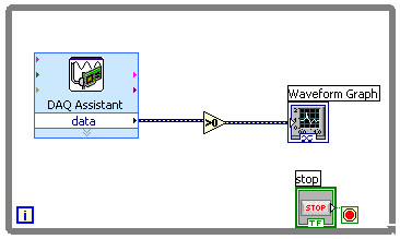
| |
Preliminary Testing: |
Turn off the under-shelf lamp to minimize the amount of noise
in the signal.
Set the function generator to produce a
20 Hz sine wave and adjust the
amplitude to produce a 1 V p-p waveform
at
Start the VI.
The waveform graph should display a 20 Hz waveform having values
of 0 and 1.
You can make the display easier to interpret by changing the Y-axis scale.
Turn off auto-scale by right clicking over the display
and selecting
AutoScale Y.
Double click on the "1" at the top of the y-axis scale and enter "2".
Enter "-2" as the lower limit.
You should now be able to clearly see the tops and bottoms of the
square wave.
| |
Viewing Input and Output Together: |
It would be nice to be able to see the original analog input as well as the
binary output.
We could add a second waveform graph to the front panel
and connect it to the A/D output.
We can also display both signals on the same graph by combining
them into a two signal vector, like we saw in Lab 4.
We can do this by using the reverse of the
Split Signals
block, called
Combine Signals.
Stop the VI and go to the block diagram. Remove the wire between the >0 symbol and the waveform graph icon and place a Combine Signals block in the resulting space (it's next to the Split Signals block in the Sig Manip palette). Connect its output to the waveform graph, its upper input to the A/D output, and its lower input to the >0 output. When you're done it should look like this: 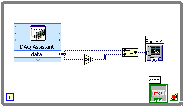
Restart the VI.
You should now see both signals, one in white and the other in red.
| |
A Variable Threshold: |
The >0 block compares its input with a fixed thershold of zero.
This is fine for converting sine waves to square waves, but in general
we would like to be able to adjust the threshold to suit our requirements.
Fortunately this is easy to do.
On the front panel, place a vertical slider and set the limits to 1 and -1. On the block diagram remove the >0 symbol and replace it with a Greater ? block. Connect its upper input and output to the dangling wires where the >0 block was removed. Connect its lower input to the output of the slider's icon. Restart the VI and verify that you can now adjust the comparator threshold. |
|
| ||
Connections: |
Since the state (blocked or unblocked) of the beam
is a DC signal, we will need to bypass the DC blocking
function in our photodiode amplifier.
The easiest way to do this is to connect the A/D input
to the output of the first stage of the amplifier, ![\includegraphics[scale=0.500000]{ckt7.2.3.ps}](img279.png)
Since we need a constant intensity light beam,
disconnect the function generator from the microphone mixer.
| |
Testing: |
With your circuit rewired as shown above, turn everything on.
Measure the value of |
There are a number of things we could do. Since we are now experts on filtering, we could filter the signal. Another approach is to use a Schmitt trigger which automatically switches between two thresholds depending on whether the signal is increasing or decreasing. If the spacing (or hysterisis) between these two levels is greater than the amplitude of the noise, only the larger excursions caused by the signal will result in changes in the output.
Rather than build up this new functionality bit by bit, we'll once again take advantage of an existing Labview program which already has it installed.
|
| ||
Setup: |
Stop the current VI and load the "Binary"
VI from the ELEC 243 program menu. This VI has
the same connections, so no rewiring is necessary.
| |
Testing: |
Select
None
from the filter select tabs (the upper set)
and
Threshold
from the lower set of tabs.
Set the threshold to the same value used in the
previous Part.
Start the VI and observe that the behavior is the same.
(To allow for smaller input signals, this VI uses separate
graphs for input, filtered input, and output.)
| |
Schmitt Trigger: |
Select
Schmitt
from the comparator tabs.
Set the threshold to the same value as the previous step
and set
Hysterisis
to approximately 25% of the threshold value.
This should result in cleaner transitions of the output waveform,
independent of the speed of the object.
| |
Observations: |
Experiment with various combinations of filter and comparator, filter parameters and threshold values, fast and slow motion, etc. Summarize the results of your experiments. |
This conversion could be applied after the comparison, using a From DDT block as we did before, with the output type being a binary vector. Alternately, we could convert the dynamic data type to an ordinary, floating point vector before the comparator. When the inputs to a comparator are ordinary data types, the output is automatically binary.
|
| ||
Inside the Binary VI: |
Open the block diagram of the Binary VI.
It is similar to the Filters VI, but it has an additional
case statement block to select the comparison method.
Note the conversion from dynamic data to vector type
between the two case statements.
| |
Sub-VIs: |
Examine the pages of the right-hand case statement.
The
Threshold
page is similar to what we constructed in Part 1,
but the
Schmitt
block contains a magic box labeled "S.T." (for "Schmitt Trigger").
This is a
sub-vi,
a connection of blocks and connections that have been
moved to a separate file to reduce clutter in the main
VI and to allow convenient reuse.
To see what's inside, simply double click over the box.
| |
The Schmitt Trigger VI: |
Connections to sub-VIs are made via controls and indicators,
so the front panel of the Schmitt trigger indicates its
input/output structure.
There are three inputs (signal, threshold, and hysterisis)
and one output (binary signal).
The block diagram is somewhat more interesting. We can see the icons corresponding to the input and output terminals, but the main feature is the strange looking block containing the functional blocks. This is a for loop. 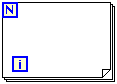
When a signal passes between the outside and inside of a block, the point of penetration is called a tunnel, denoted by the small square on the border of the block. When an input (or output) to a for loop is a vector, it exhibits a useful property called auto-indexing. In this case, the loop limit (N) is taken from the dimension of the vector, and on the inside of the loop, the value of each signal is the i-th component (a scalar) rather than the entire vector. This allows us to do point-by-point operations on a vector. Another useful property of a for loop is the ability to pass a value from one iteration of the loop to the next. This is done by using a shift register, denoted by a small rectangle with an upward pointing arrow on the right hand border and a corresponding node with a downward pointing arrow on the left border. 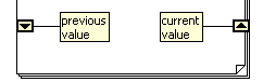
| |
Observations: |
Examine the S. T. VI and convince yourself that it does indeed implement a comparator with hysterisis. |
If the amplitude of the noise is small compared to the difference between the blocked and unblocked photodiode output, the techniques described above will work reliably. This is the case for our optical interrupter, where the distance between the emitter and detector is small compared to the distance to the sources of interference. However, as we increase the separation between emitter and detector, the amplitude of the signal from the emitter will decrease while that from the interference will remain the same. Eventually the system will fail.
The way to improve the situation is to increase the signal to noise ratio. Since the signal characteristics of the noise are fixed, we should choose an emitter signal that can be successfully separated from the noise by filtering. In our situation, most of the noise is due to ambient lighting. For some sources, this includes a strong periodic component at multiples of 60 Hz, but in all cases it includes a significant DC component. This means the signal from the emitter should be at a high frequency, preferably an odd multiple of 30 Hz.
If we use an AC signal for the emitter signal, we can no longer compare the received signal from the detector to a threshold to determine if the beam is blocked or unblocked. If we did, it would appear that it was being interrupted at the modulating frequency. Instead, we need to apply the threshold to the amplitude of the filtered detector waveform. There are a number of ways we can determine this amplitude. The simplest is to simply take the absolute value and smooth the result with a low pass filter. This is the same process used to receive AM radio stations, and is called envelope detection.
|
| ||
Setup: |
Reconnect the A/D input to ![\includegraphics[scale=0.500000]{ckt7.2.4.ps}](img280.png)
Set the function generator frequency to the value
determined in Part 6 of Experiment 9.1.
Set the filter tab to
AM.
Set the
Frequency
slider to the function generator frequency
and the
Bandwidth
to 200 Hz.
Measure the
Output RMS
with the beam blocked and unblocked and
set the
Threshold
halfway between the two values.
| |
Testing: |
Verify that the
Output
corresponds accurately to the
blocked/unblocked state of the beam.
| |
Observations: |
Simulate increasing distance between the emitter and detector by reducing the function generator output. Adjust the Threshold appropriately. How low can you get and still achieve reliable operation? To what increase in distance does this correspond? |
In some cases all we need to know is whether or not something is positioned between the emitter and detector or the optical interrupter. However, sometimes we need to know more quantitative information. For example, how long was it there, how many times was it there, etc? We can get this information by counting the output pulses, measuring their width, etc.
Labview provides several VIs for working with pulses which can tell us things such as their rate and width. Other functions, such as counting pulses, we will have to build ourselves. One such VI, which counts the number of 0-to-1 transitions, has been built and installed in the Process program. Its results are displayed in the numeric indicator labeled Count in the lower right quadrant of the front panel. The adjacent Reset button restores the count to zero.
|
| ||
Setup: |
Use the setup from either Part 2 or Part 5
of this Experiment.
| |
Testing: |
Using an appropriate opaque object, block and unblock the beam.
Verify that the count increases by one each time the object passes
through the beam.
| |
Observations: |
Examine the count VI.
Write a brief summary of how it works.
| |
Design Challenge: |
Create a Labview program that displays the total amount of time that the beam has been blocked. Include a button to reset the total. You can either create the program from scratch or start with the Binary program and add the additional functionality. If you do the latter, save a copy to your own directory before starting and work from that copy. |