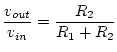
![\includegraphics[scale=0.650000]{voltage_div.ps}](img256.png)
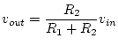
The following figure shows the basic voltage divider circuit:
 or
or
If we replace resistances ![]() and
and ![]() by impedances
by impedances
![]() and
and ![]() and use the phasor representation
(
and use the phasor representation
(![]() and
and ![]() ) for the input and output voltages,
then the voltage divider relation still holds.
We define the ratio of the output voltage phasor to the input
voltage phasor to be the
transfer function:
) for the input and output voltages,
then the voltage divider relation still holds.
We define the ratio of the output voltage phasor to the input
voltage phasor to be the
transfer function:
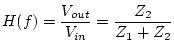
For example if we replace ![]() with a capacitor, we get the following
circuit:
with a capacitor, we get the following
circuit:
![\includegraphics[scale=0.650000]{low_pass_phasor.ps}](img257.png)
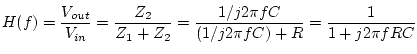
Since ![]() is close to unity for small values of
is close to unity for small values of ![]() and goes to
zero for large
and goes to
zero for large ![]() (i.e. it passes low frequencies
and attenuates high frequencies)
we call this circuit a
low pass filter.
(i.e. it passes low frequencies
and attenuates high frequencies)
we call this circuit a
low pass filter.
Since the transfer function describes how effective a system
at transmitting
(or blocking)
sinusoids of a particular frequency, it is also referred to as the
frequency response.
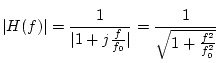
Note that ![]() is complex.
If we want to work with
quantities we can measure in the lab, i.e.
real numbers, we can
express
is complex.
If we want to work with
quantities we can measure in the lab, i.e.
real numbers, we can
express ![]() in polar form in terms of its
magnitude
(
in polar form in terms of its
magnitude
(
 ).
and
phase
(
).
and
phase
(
![]() ).
).
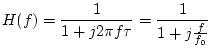
We can simplify the transfer function of the system above by
defining the
time constant
![]() and the
cutoff frequency
and the
cutoff frequency
![]() ,
which gives
,
which gives
![\includegraphics[scale=0.350000]{fr1.ps}](img258.png)
Why logarithmic?
The smallest perceivable sound level corresponds to an acoustic
power density of approximately
![]() .
But the level at which the sensation of sound begins to give way
to the sensation of pain is about
.
But the level at which the sensation of sound begins to give way
to the sensation of pain is about ![]() .
To cope with this large dynamic range without loosing track of
the number of zeros after the decimal point, a logarithmic
scale is useful.
.
To cope with this large dynamic range without loosing track of
the number of zeros after the decimal point, a logarithmic
scale is useful.
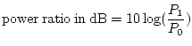
It's important to remember that a decibel measurement expresses a
ratio.
So it always makes sense to say that a signal x is so many dB
greater (or less) than signal y.
But if we say that a signal is
equal
to some number of decibels, then there must be a reference level.
For sound, that reference level is usually taken as
![]() which corresponds to a pressure of
which corresponds to a pressure of
![]() .
If we call this the reference pressure level,
.
If we call this the reference pressure level, ![]() ,
we get the definition of
sound pressure level
,
we get the definition of
sound pressure level
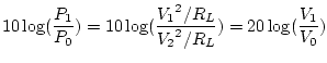
In a circuit, the choice of a reference level is not quite so obvious. For voltages, the typical choice is 1 V, which gives "decibels relative to 1 Volt" or dBV for short. Other forms you may encounter are dBW (relative to 1 watt) or dBm (relative to 1 mW).
It is sometimes stated that the response of a filter falls off at
"20dB per decade" or "6dB per octave".
This is just another way of saying that the response varies as 1/f.
In other words, if ![]() is 10 times
is 10 times ![]() (i.e. the frequencies are
separated by one decade) then
(i.e. the frequencies are
separated by one decade) then ![]() will be 1/10 of
will be 1/10 of ![]() .
Since
.
Since
![]() then we have a loss of 20dB (or a gain
of -20dB) for each decade increase in frequency.
Similarly, for two frequencies separated by one octave (a factor of
two) we would have
then we have a loss of 20dB (or a gain
of -20dB) for each decade increase in frequency.
Similarly, for two frequencies separated by one octave (a factor of
two) we would have
![]() or approximately 6dB per
octave.
or approximately 6dB per
octave.
If we plot the amplitude of the frequency response in dB
vs ![]() we get what's called a
Bode Plot
(named after Hendrick Bode who devised this method of
representation at Bell Labs in the 1940s).
we get what's called a
Bode Plot
(named after Hendrick Bode who devised this method of
representation at Bell Labs in the 1940s).
![\includegraphics[scale=0.350000]{fr3.ps}](img259.png)