ELEC 332

In the Lab

This week in the lab we will play with two types of sensors, resistive and piezoelectric. Resistive sensors were discussed in the Background section and a resistive sensor is the subject of this week's design challenge. In the structured part of the lab we will look at two piezoelectric transducers: a vibration sensor and an ultrasonic transceiver.

A piezoelectric material is one in which the electric polarization changes in response to mechanical strain. Commonly used materials include crystals (e.g. quartz), ceramics (e.g. barium titanate), and polymers (e.g. polyvinylidene fluoride (PVDF)). A typical transducer consists of a thin piece of piezoelectric material with a conductive electrode on each surface. When deformed, the change in polarization is manifest as a variation in surface charge, which results in an electric field within the material, which appears as a voltage at the electrodes. In other words, the device looks like a capacitor whose charge is a function of mechanical strain.

This effect works in reverse: applying a voltage to the electrodes establishes an electric field in the material, which in turn produces a mechanical stress. This stress will interact with the elastic properties of the material to produce a corresponding strain or mechanical motion.

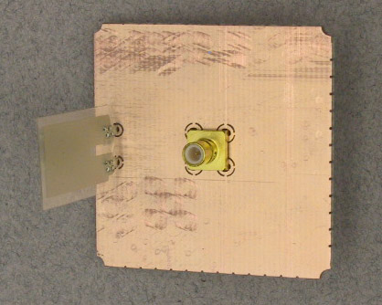
Part 1: Piezoelectric Vibration Sensor

The LDT Vibration Sensor consists of a piece of piezoelectric film which produces a voltage when bent, or which will bend when a voltage is applied.

Measure response to bending.
We could just hold the sensor in the clip leads to test it, but soldering it to a breadboard module gives a more controlled environment.
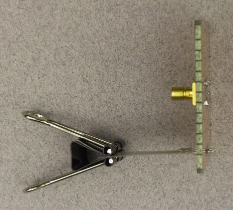
(Click to enlarge) Mount the module on the breadboard, using all four screws to provide stable support. Connect the sensor output to the oscilloscope. Gently bend the strip back and forth. Describe the resulting output.

Measure response to vibration.
Subject the breadboard to mechanical vibration. Describe the resulting output. Low frequency sensitivity can be increased, at the expense of high frequency response, by adding mass to the free end of the sensor. Clamp a small binder clip to the tip of the sensor and apply the vibration again.
(Click to enlarge) Describe the difference in response with and without the additional mass.

Use as a microphone.
Since our sensor has a significant area, it should be able to respond to vibrations in the atmosphere, i.e. sound waves. Remove the binder clip used in the previous step to restore high frequency sensitivity. Speak, whistle, play a trumpet, or otherwise direct an acoustic signal toward the sensor and observe the resulting output.

Use as a speaker.
Since the piezoelectric effect works in reverse, we should be able to use our vibration sensor as a vibration producer. Disconnect the sensor from the oscilloscope and connect it to the function generator. Apply sinusoidal inputs of various frequencies and observe the response.

Part 2: Charge Amplifier

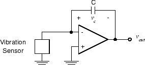
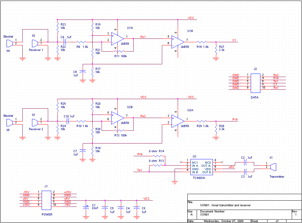
One problem with trying to measure the voltage produced by a piezoelectric sensor is that the finite input impedance of the measurement device (the oscilloscope in our case) rapidly drains the charge from the capacitor and the output decays to zero. For AC signals above the cutoff frequency of the resulting high pass filter, this isn't a problem, but if we want to measure low frequency or static displacements, we need a very high or infinite input impedance. Infinite impedances are hard to come by, but we can get a very large one by using a FET input op amp, such as the LF411.

We could configure the LF411 as a voltage follower and use it as a buffer, but high impedances are susceptable to noise pickup. A better approach is to remove the charge from the sensor (via a very low impedance connection) and place it on another capacitor. If we connect the vibration sensor as shown in Fig. 1 the charge will flow into the summing junction of the op-amp and be transfered to the capacitor. Because of the extremely high input resistance of the LF411 op-amp, it will take a much longer time for this charge to leak away.

Fig. 1: Charge Amplifier To prevent offsets and bias currents from saturating the circuit, a large leak resistor is usually added as shown in Fig. 2.

Fig. 2: Leaky Charge Amplifier This circuit has been realized on the second of this week's modules:

(Click to enlarge)

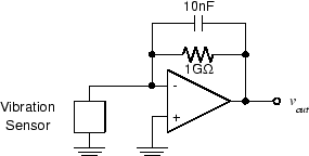
Up to now all of our modules have used surface mount components. 1 GΩ resistors aren't available in surface mount packages, and we had some LF411s available in DIP packages, so this module provides an example of how to use thru-hole components with our milled PC boards. Note that several of the leads are soldered on both sides of the board to provide a via function.

Vibration:
Repeat the vibration and microphone measurements from the previous section. Compare the results with and without the charge amplifier.

Low
Move the tip of the vibration sensor back and forth while observing v_out. You should see a voltage which is proportional to the deflection.

Displacement:
Release the sensor and allow v_out to stabilize. Move the tip of the sensor a few millimeters and hold it in position. How long does it take for the output to decay back to zero. What happens when you release the sensor?
Allow v_out to stabilize again, then move the tip exactly 10 mm. Measure the resulting output voltage.

Acceleration:
Attach the binder clip as in the previous section. Allow the output to stabilize, then tilt the breadboard assembly and observe the output.

Part 3: Sonar Rangefinder

Piezoelectric devices made from crystaline materials are high Q mechanical resonators. The quartz crystal oscillator in your watch or clock makes use of this property to produce a very accurate frequency reference. In a sensor, resonance is usually undesirable, but for narrowband applications, the associated increase in sensitivity can be useful. One such application is ultrasonic ranging, where a short burst of high frequency sound is reflected from a surface and the delay of the echo is used to determine the distance. Since this frequency is fixed, a resonant transmitter and receiver provide high sensitivity at low cost.

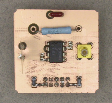
Our third module for this week utilizes such transducers to generate and receive the pulses, some circuitry to drive the transmitter and amplify the received signal, and the MSP430 to generate the pulse.

(Click to enlarge)

As with the motor driver of Exercise 4, this circuit has several options which may be selected by jumpers or choice of installed components. It is currently wired with a piezoelectric receiver on the left hand side and an electret microphone on the right. This allows us to compare the sensitivity of the resonant receiver with that of a broadband transducer.

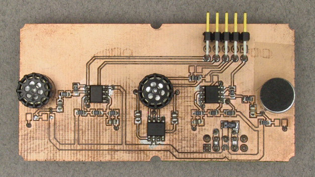
Connect the modules.

We have a new connector module which allows us to monitor the signals between the MSP430 and the sonar transciever.

(Click to enlarge)
When it's all put together, it looks like this: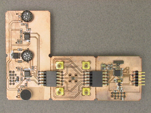

(Click to enlarge) Note that to allow the receivers to be symmetrically placed at the two ends of the module, it was necessary to put the interface connector on the top of the board, rather than the left hand side. This results in a right angle bend in our normal straight line flow of connectivity.

Connect the scope.
Using the SMB connectors on the intermediate module, connect channel 1 of the scope to the transmitter drive signal on P1.4 (the connector in the lower left corner). Connect channel 2 to the receiver output signal Rx1 (upper right corner). Set the scope to trigger on channel 1.

Build, load, and run the program.
Compile, load, and run the program lab6.c from this week's zip file. The green LED on the CPU board should come on.

Look at the signals.
Set the time time base to about 50 µs per division. You should see 8 cycles of a 40 kHz square wave on the transmitter drive. Set the time base to about 2 ms per division. You should see a large burst on the receiver output immediately after the transmitter burst. Set channel 2 to AC coupling and increase the gain until you can see the echo of the ceiling at about 12 ms. Use dual sweep with delayed trigger to get a closer look at the echo.
Place various objects in the path of the beam, move them up and down, and observe the resulting echoes.
Move channel 2 to the comparator output (upper left connector) set the gain back to 2 V/div, and the coupling back to DC. Is the ceiling echo detected? Place and move other objects above the beam and assess how effective the comparator output is in determining their distance.


Measure response to bending.		We could just hold the sensor in the clip leads to test it, but soldering it to a breadboard module gives a more controlled environment. (Click to enlarge) Mount the module on the breadboard, using all four screws to provide stable support. Connect the sensor output to the oscilloscope. Gently bend the strip back and forth. Describe the resulting output.
Measure response to vibration.		Subject the breadboard to mechanical vibration. Describe the resulting output. Low frequency sensitivity can be increased, at the expense of high frequency response, by adding mass to the free end of the sensor. Clamp a small binder clip to the tip of the sensor and apply the vibration again. (Click to enlarge) Describe the difference in response with and without the additional mass.
Use as a microphone.		Since our sensor has a significant area, it should be able to respond to vibrations in the atmosphere, i.e. sound waves. Remove the binder clip used in the previous step to restore high frequency sensitivity. Speak, whistle, play a trumpet, or otherwise direct an acoustic signal toward the sensor and observe the resulting output.
Use as a speaker.		Since the piezoelectric effect works in reverse, we should be able to use our vibration sensor as a vibration producer. Disconnect the sensor from the oscilloscope and connect it to the function generator. Apply sinusoidal inputs of various frequencies and observe the response.


Vibration:		Repeat the vibration and microphone measurements from the previous section. Compare the results with and without the charge amplifier.
Low		Move the tip of the vibration sensor back and forth while observing v_out. You should see a voltage which is proportional to the deflection.
Displacement:		Release the sensor and allow v_out to stabilize. Move the tip of the sensor a few millimeters and hold it in position. How long does it take for the output to decay back to zero. What happens when you release the sensor? Allow v_out to stabilize again, then move the tip exactly 10 mm. Measure the resulting output voltage.
Acceleration:		Attach the binder clip as in the previous section. Allow the output to stabilize, then tilt the breadboard assembly and observe the output.


Connect the modules.		We have a new connector module which allows us to monitor the signals between the MSP430 and the sonar transciever. (Click to enlarge) When it's all put together, it looks like this: (Click to enlarge) Note that to allow the receivers to be symmetrically placed at the two ends of the module, it was necessary to put the interface connector on the top of the board, rather than the left hand side. This results in a right angle bend in our normal straight line flow of connectivity.
Connect the scope.		Using the SMB connectors on the intermediate module, connect channel 1 of the scope to the transmitter drive signal on P1.4 (the connector in the lower left corner). Connect channel 2 to the receiver output signal Rx1 (upper right corner). Set the scope to trigger on channel 1.
Build, load, and run the program.		Compile, load, and run the program lab6.c from this week's zip file. The green LED on the CPU board should come on.
Look at the signals.		Set the time time base to about 50 µs per division. You should see 8 cycles of a 40 kHz square wave on the transmitter drive. Set the time base to about 2 ms per division. You should see a large burst on the receiver output immediately after the transmitter burst. Set channel 2 to AC coupling and increase the gain until you can see the echo of the ceiling at about 12 ms. Use dual sweep with delayed trigger to get a closer look at the echo. Place various objects in the path of the beam, move them up and down, and observe the resulting echoes. Move channel 2 to the comparator output (upper left connector) set the gain back to 2 V/div, and the coupling back to DC. Is the ceiling echo detected? Place and move other objects above the beam and assess how effective the comparator output is in determining their distance.