| |
|

|
Initial Configuration |
|
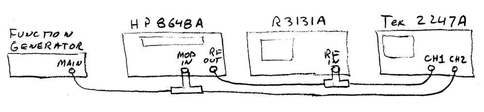
Connect together the scope, signal generator, spectrum analyzer, and Wavetek
function generator as shown in the diagram,
using BNC Tees and coax cables.
The purpose is to view the signal generator output on both the scope and the
spectrum analyzer.
The function generator is used to provide a modulating waveform
(the builtin 400 Hz and 1 kHz modulating signals are two low in
frequency to produce visible AM sidebands on the spectrum analyzer).
(Click to enlarge)
Set the function generator to produce a 10 kHz, 2.5 V sine wave.
|
Initializing: |
|
When the spectrum analyzer is turned on, it returns to its previous configuration.
Since the spectrum analyzer has a large number of settings, some of which can cause
it to do distinctly odd things, it's a good idea to start by returning it to
some sort of "normal" configuration before starting.
Fortunately, most of the settings are displayed on the screen,
so we can check the configuration quickly if we know what to look for.
Here's what we want
(starting at the upper left of the screen):
- REF
-
Should be 0.0 dBm. If not: press the
LEVEL
button, enter
0
on the numeric keypad, and press the
GHz +dBm dB
key.
- ATT
-
Should be 10dB.
If not: press the
LEVEL
key, then use the
ATT
soft key to select
AUTO.
- A_wrt
-
If this says A_avg, A_blnk, or something else:
press the
TRACE
key,
then press the
Write A
soft key.
- B_blnk
-
If something else is displayed in this position:
press the
TRACE
key, the
Trc Menu A/B
key, and
Blank B.
Verify that the bandwidth is in the automatic mode:
Press the
BW
key,
then use the soft keys to insure that both
RBW
and
VBW
have
AUTO
selected.
|
Observing a signal: |
|
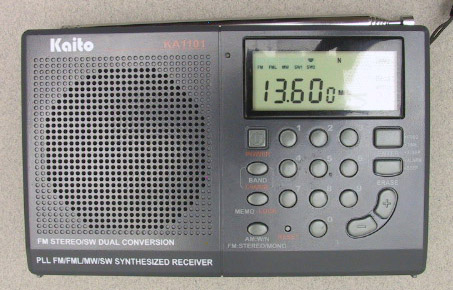
Set the signal generator to produce a 10 MHz, -10 dBm, unmodulated signal.
Set the spectrum analyzer to a center frequency of 10 MHz and a span of 1 MHz.
We would expect to see a single line in the center of the display, but what we
actually get looks more like a tent.
This is because the bandwidth chosen in the automatic mode is fairly wide, to provide
for a fast sweep rate.
Try changing the span size and notice that the bandwidth
(labeled
RBW
(for Resolution Bandwidth) at the bottom of the screen)
also changes, keeping the shape of the display roughly the same.
|
Changing the bandwidth: |
|
We can get a more line-like display by reducing the bandwidth.
To do this, press the
BW
key, then use the softkeys to set the
RBW
mode to
MNL
(manual).
Use the knob or the arrow keys to decrease the bandwith and note how the
display changes.
The lowest available bandwidth is 1 kHz.
This is the 3 dB bandwidth, so the width of the "spike" at its base will
be significantly wider.
|
Using the marker: |
|
Set the
SPAN
to 100 kHz
and the
BW
to 1 kHz.
Press
PK SRCH
key under
MARKER
to set the marker to the peak value.
The frequency and amplitude of the marker are displayed in the upper right
portion of the screen.
Comment on the accuracy of single frequency measurement with the spectrum analyzer.
|
Resolving signals: |
|
Set the function generator as specified in the initial configuration
(10 kHz, 2.5 Vpp sine wave).
Set the signal generator modulation to extenal AC and turn the modulation on.
You should see the two sidebands 10 kHz to either side of the carrier
frequency.
The additional sidebands are due to the fact that the sine wave output of the
function generator is not very accurate, so there is significant harmonic distortion.
To see lots of harmonics, briefly set the function generator to square wave.
Return the function generator output to sine wave, and change the frequency
to 1 kHz.
We would expect to see sidebands 1 kHz either size of 10 MHz, but because
of the limited resolution of the spectrum analyzer, all we see is a mess.
The moral: be careful in interpreting what you see on the spectrum analyzer.
|
Small signals: |
|
Reduce the signal generator output in steps of 10 dBm while watching the
signal on both the scope and the spectrum analyzer.
Adjust the
Volts/div
of the scope and the
LEVEL
of the spectrum analyzer as necessary to maintain a satisfactory display.
|
Using averaging: |
|
As you reduce the reference level, you will start to see a fuzzy band
(sometimes called
grass)
at the
bottom of the display. This is noise, both on the input signal, and internal to the
spectrum analyzer.
To see how much of the noise is internal, temporarily unplug the input connector.
Since the noise is random, its effect can be reduced by averaging.
To turn on averaging, press the
TRACE
key, use the bottom soft key to select the second half of the trace menu,
press the
AVG A
key and turn averaging
ON.
This should significantly reduce the amplitude of the noise, while leaving the
input signal undisturbed.
Continue reducing the amplitude of the input until it is no longer possible to
detect it.
Comment on the magnitude of the minimum detectable signal for both the scope
and the spectrum analyzer.
|
| |
|
|
Setting up: |
|
Set the spectrum analyzer to the following configuration:
reference level (REF)
0.0 dBm,
center frequency 100 MHz,
span 200 MHz,
bandwidth automatic,
averaging off.
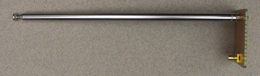
Remove the coax cable from the spectrum analyzer input and replace it with
a banana plug to BNC adapter. Fully extend one of the whip antennas and plug
it into the red terminal of the adapter.
With a little care, friction will hold the antenna in the vertical direction
(it helps to rotate the adapter so that the red terminal is on the bottom).
|
Signals in the lab: |
|
You should see a bump just to the left of the center of the screen.
This is the FM broadcast band.
These are the only signals with the proper combination of power and wavelength
to be able to penetrate deep into the interior of the building where the lab is
located.
However, there are plenty of signals originating inside the building which can be
picked up, mostly originating from the large number of switching power supplies
in the lab and in surrounding rooms.
This cacophony usually blends together into a random looking noise, but
by touching the antenna or moving it to a different orientation, you may be
able to pick up some individual signals (recognizable by their
regularly spaced harmonics).
There's another signal of much higher frequency that we can pick up.
Set the spectrum analyzer center frequency to 2.4 GHz, and the span to
500 MHz.
Return the whip antenna to the vertical position.
Turn on the microwave oven.
|
Signals outside the lab: |
|
Fortunately we have some antennas outside the building which can pick up
a better selection of interesting signals.
Return the spectrum analyzer settings to 100 MHz center frequency,
200 MHz span.
Remove the whip antenna and banana plug adapter.
Plug in the outside antenna cable (marked with a piece of blue tape).
You should now see a number of bumps.
The FM band is still there, with significantly higher amplitude.
The hump at the far left is the AM broadcast band and the international
shortwave broadcast bands. The pair of spikes around 60 MHz is Channel 2.
Channel 8 and Channel 13 are near the right side of the display, and you
may be able to see some pager and two-way radio traffic around 150 MHz.
Try using the
FREQUENCY,
SPAN,
and
BW,
controls to zoom in on some of these signals.
|
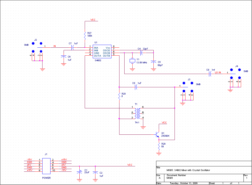
The mixer we will use is the
SA602, which is based on a Gilbert Cell
multiplier.
This is a fully differential circuit,
but there are various ways of using it with single ended signals,
including simply ignoring one of the inputs or outputs.
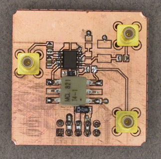
We will be using two different modules, each with a different configuration.
The first has an external oscillator input, no offset on the baseband input,
and a transformer coupled output.
Since there is no offset added to the input, the output will be of the form
x(t) = A s(t)cos(ωct)
where ωc is the frequency of the
external oscillator.
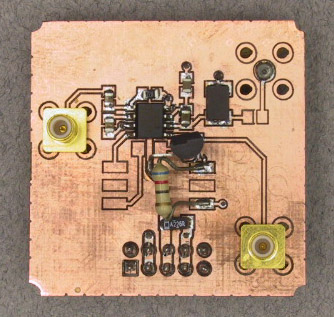
The second has an on board 13.56 MHz crystal oscillator,
adds an offset to the modulating input to produce AM,
and has an emitter follower output buffer.
Because of the offset, the output is
x(t) = A (s(t)+1)cos(ωct)