ELEC 432

---

When we use Labview to simulate a system or test a concept we can connect a signal generator block to the input, a waveform display to the output, and press RUN. If we want to use real world analog inputs and outputs, things get a bit more complicated. Commands must be issued to configure and start the hardware, interrupts must be handled, data must be collected into blocks and delivered to the appropriate process, and error conditions such as buffer overflow or underrun must be detected and handled. Fortunately, Labview takes care of most of the details for us, but we still need to be aware of what's going on in the background and occasionaly help it along.

Part 1: Analog I/O with the Sound Card

There are two shortcomings to sound card access in Labview:

1. There are no Express VIs available, so a set of low level VIs must be used.
2. Resolution is limited to 16 bits and maximum sample rate to 44.1 kHz, even if the sound card is capable of more.

Selecting the sound card:		Sound cards are identified in Labview by a device number. The safest way to select from among multiple available cards is to set the device number to zero, which specifies the default sound card, and use the Sounds and Audio Devices control panel to select the default. To do this: Open the Sound and Audio Devices control panel. Select the Audio tab. Select either Soundmax Digital Audio or M-Audio Delta 44 Multi as the default device for both Sound playback and Sound recording. Press Apply. 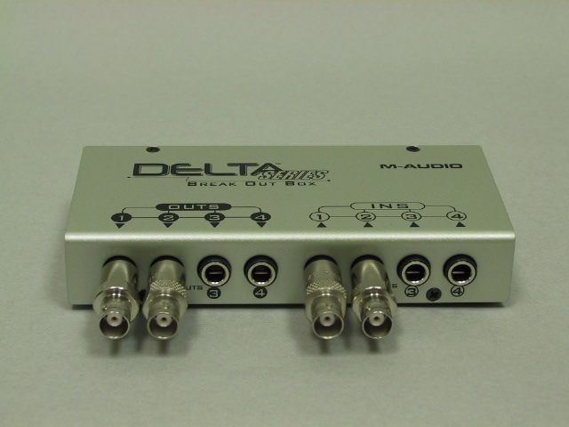The M-Audio card is more convenient since there are 1/4" phone plug adapters in the break-out box that allow for direct connection of BNC cables.
Sound card input:		Load the sound card input example VI: sc_in.vi. Select Show Block Diagram from the Window menu to display the block diagram. The functions of the SI CONFIG and SI START VIs must be performed once before conversion begins, and the SI CLEAR must be called when conversion is complete, so these are placed outside the loop. Each time the SI READ VI is called it outputs one block (of size Buffer Size) of samples. The thin blue wires (task ID) and the stripped pink wires (error) which chain the VIs together provide the data flow dependency to insure that they are called in the proper sequence. This VI does nothing with the samples except to display them on a waveform chart. Connect the function generator to input channel 1 and verify that the VI is working properly.
Sound card output:		Load the sound card output example VI: sc_out.vi and examine its block diagram. This VI produces a sine wave and sends it to the sound card output, as well as displaying it on the front panel. Note the SO WAIT VI. When reading from the sound card input, the rate at which samples are acquired limits the rate of execution of the rest of the VI. The waveform generator can produce samples at a much faster rate than the sound card output can dispose of them, so to prevent running out of memory trying to store all these samples, the SO WAIT VI blocks execution until the sound card has consumed all the samples in its current block. Connect output channel 1 from the sound card to the scope and observe the output signal.
Combined input and output:		Load the VI: sc_inout.vi which combines input and output. Examine the block diagram, noting that since the input now controls the rate of execution, the SO WAIT block is no longer needed. This VI does nothing but connect the input directly to the output, but to make it slightly more interesting, it now does it in stereo (note the doubled line between SI READ and SI WRITE denoting a 2-D array. Run this VI with the input connected to the function generator and the output connected to the scope and verify that is working correctly.

Part 2: Displaying Data

Waveform charts and graphs have a number of options to control the display of data. These may be accesed by right clicking over the front panel indicator while the VI is stopped. The location at which you click is important: clicking over an axis selects options for that axis, clicking over the display area displays options for the entire display, with sub-menus for the axes. Experiment with the options (in conjunction with the User's Manual and Help files if your sense of adventure becomes overtaxed).

Part 3: Basic Processing

Simply reading samples of a signal and sending them directly to the output is not very exciting, the same function could be performed with a piece of wire. The whole point of DSP is to process the signals, so let's get started doing that.

Load the VI:		Load the sc_proc VI and open its block diagram.
Express VIs:		The big blue VI labeled "Filter" is an Express VI. This is a type of high-level function block with a wizard-style user interface. Express VIs can make building a Labview program easier, although the associated overhead does incur a performance penalty. Express VIs operate on dynamic data types (denoted by the striped dark blue wire). Note the Convert to Dynamic Data and Convert from Dynamic Data blocks on the input and output of the filter block. These are necessary to interface the Express VI with the "ordinary" VIs making up the rest of the program. These are not always necessary, as many non-express VIs are capable of handling the dynamic data type. When in doubt, try a direct connection, and if the resulting wire is a black dashed line (indicating an error), add the appropriate conversion.
Filtering:		Using the connection left over from the previous steps (input from function generator, output to scope) run the VI and observe that the output is indeed an appropriately lowpass filtered version of the output. (The Frequency control is labeled in the fraction of the sample rate, not Hz.)
Different Filtering:		Double click on the Filter VI to bring up the Configure Filter dialog. Try various different types of filters and observe the results.

Part 4: Digital Radio Breadboard

So far we've been able to make all of our interconnections with BNC cables, since everything we wanted to connect either had BNC connectors on it, or we could find a BNC adapter for the type of connectors that it had. Although a BNC breakout box is available for the NI 6251 DAQ card, we have chosen a more flexible route, similar to what we have done in 241 and 242 lab, i.e. build a breadboard/interface module system for constructing our circuits and accessing their inputs and outputs.

In fact, we could use the new 241/242 breadboard since it has all the necessary connectors (and if it didn't we could build an additional module that did). However this would be unsatisfactory because

1. Most of the the chips we will want to use only come in surface mount packages.
2. Even if we made adapters for them, the grounding and shielding limititations would cause us to pick up and radiate too much noise.

1. The modules are smaller, so that we can have more of them.
2. Each module has its own power supply regulators.
3. Instead of the solderless breadboard strips, prototyping techniques are used which allow for the use of surface mount components and provide a good ground plane.
4. All of the jumpers are coax rather than unshielded wire.

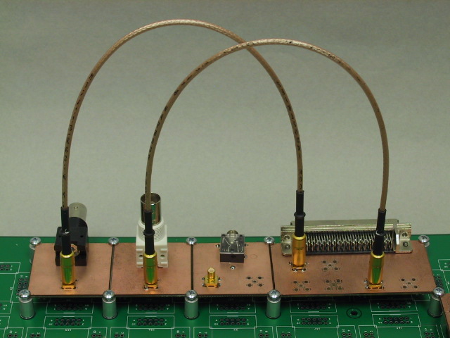
For this exercise, all we need is the ability to connect to the NI 6251 cable, so we will use only a few of the connector modules This picture shows Channel 0 of the A/D converter connected to the black BNC connector and Channel 0 of the D/A converter connected to the white BNC connector, which is the configuration we will use in the first part of the lab.

The small, gold coax jumper connectors are SMB type connectors. SMB connectors are push-on, so no rotation is required, just a strong push or pull.

Set up connections:		If the breadboard is not set up as shown in the picture, use SMB coax jumpers to connect the black BNC connector to the left hand plug on the DAQ module and the white BNC connector to the left-most plug on the DAQ module. Connect the RF signal generator to the A/D input (black BNC) and the scope to the D/A output (white BNC).
Terminate the A/D input:		The A/D inputs to the DAQ card have a very high input impedance. Unless a low impedance DC path to ground is provided, an offset potential will build up and drive the input into saturation. The signal generator has a capacitor coupled output, so be sure use a BNC-T with a terminator resistor at the connection to the A/D input.

Part 5: Analog I/O with the NI 6251

For the NI 6251 data acquisition card, Express VIs are available to eliminate the need for low level VIs. To avoid terminal boredom, we will skip over input-only and output-only versions and go directly to a combined input and output shell.

Download a sub-VI:		The VIs used in this and subsequent parts require a sub-vi: daq2. Download and save this VI.
Load the VI:		The input/output VI shell for the 6251 is ni_inout. You can either download and save this to the same directory as the sub-vi, or run it directly from the browser link, in which case it will ask you where you saved daq2.vi. (Ignore the message telling you that it found daq2.vi in a different place than it expected to find it.) When it is loaded, display the block diagram.
Converting express to regular VIs:		The analog input VI (daq2.vi) was initially a DAQ Assistant Express VI, but has been converted to a regular VI and modified to allow external control of the channel, sampling rate, and block size (hence the yellow rather than blue background). If you wish to do this with other Express VIs, right click on the VI and select Open Front Panel.
Try it out:		Set the signal generateor to 200 kHz, -30 dBm. Start the VI and observe the signal on the waveform display and the scope.
Display update rate:		With the sound card, we could display each block of samples without consuming much CPU time. With a sampling rate over 20 times faster, the overhead of displaying all the samples could consume a significant fraction of our processing capacity. By displaying only every n-th block of samples, we can significantly reduce the display overhead, and actually make the display easier to read. The control marked Display Rate does this by only enabling the waveform graph one out of every N times through the loop. Examine the block diagram to see how this works.
Observe aliasing:		Increase the signal generator frequency (say, in multiples of 100 kHz) and observe how the signal is aliased as it passes through multiples of fs/2. Since the input signal is bandlimited, with a bandwidth less than fs/2, no information is lost. However, note that as the order of aliasing is increased, the amplitude of the digitized signal decreases. Find the input frequency at which the digitized signal is 3 dB down from its unalised value.

Part 6: A Digital AM Radio

Enough messing around. Let's build something useful. Our next VI adds some processing to the ni_inout VI.

Load the VI:		The VI used in this part, ni_proc also uses the daq2 VI, so use the same procedure as in the previous part to load this VI.
The front panel:		This VI combines an AM radio receiver, a spectrum analyzer, and a waterfall display, so there's a lot going on. The block marked "Radio" contains the controls for tuning and adjusting the radio. The block marked "Input" selects the input channel and sampling parameters. These controls should not require adjustment for this exercise. The two graphs in the center display the spectrum of the input and the demodulated output waveform, respectively. The large display on the right is a waterfall display which shows how the spectrum changes with time. Frequency is plotted on the y-axis, time on the x-axis, and amplitude (the z-axis) is indicated by color: dark blue indicates low amplitude, white indicates high amplitude.
The block diagram:		Examine the block diagram. The spectrum analysis is handled by an Express VI, requiring almost no effort on our part. The waterfall display is simply a matter of connecting the spectrum to a different type of indicator (an Intensity Chart). The filtering and generation of the local oscillator waveform we've seen before. There are two separate AM detectors, an envelope detector, implemented with an absolute value block, and a direct conversion or product detector which simply multiplies the received signal by the local oscillator signal. The only new trick is the selector (the triangle with the "wishbone" in it) which is used to switch the filters in and out of the circuit and to select one of the two detector outputs.
Initial connections:		With the inputs and outputs connected as in the previous part (signal generator to input, scope to output) set the signal generator to 120 kHz, -30 dBm.
Receiving a signal:		Set the Radio group controls as follows: Carrier Frequency: 120000 Hz. Fine Tune: 0. Clarify: 0. RF Filter: 120000. Volume: 25 RF Filter (button): off. AF Filter (button): on. Detector: Envelope. Start the VI and verify that the spectrum display is what it should be.
Receiving an aliased frequency:		Set the signal generator to 1.12 MHz. The displays and output should be essentially the same as before. Adjust the signal generator frequency up and down and observe the direction in which the spectrum display moves. Set the signal generator to 880 kHz. Again move the signal generator frequency up and down and observe the direction of motion of the spectrum display.
Demodulating AM:		Return the signal generator frequency to 120 kHz. Set the signal generator modulation to internal AM, either 400 Hz or 1 kHz and turn the modulation on. Observe the demodulated waveform on the VI's waveform dispay and on the scope. Try both envelope and product detectors, AF filter both on and off. Unless the signal generator and A/D sampling clock are both exactly synchronized, it will be necessary to adjust the Clarify control (the fine fine-tuning control) to stabalize the output signal.
Receiving AM radio stations:		Disconnect the signal generator and connect the outside antenna (the cable with the blue tape) to the A/D input. Be sure to leave the terminator connected to the A/D input. Start the VI and turn the RF filter OFF. Observe the large number of spikes in the spectrum display. These are the carriers of the local AM radio stations and should be located on multiples of 10 kHz. On the waterfall display the modulation sidebands should be clearly visible.
Receiving one AM station at a time:		As long as none of the stations have aliased on top of each other, it is possible to recieve each one individually. With the envelope detector, this is done by placing a bandpass filter before the detector, centered on the desired frequency. With the product detector, the local oscillator is set to the desired frequency, shifting the signal back down to baseband. The AF filter then removes the undesired channels, which have also been shifted in frequency.
Listening to AM radio:		Move the SMB coax jumper from the module with the white BNC connector to the one with the phone jack. Plug a speaker into the phone jack and turn it on. Try tuning in a few stations using both the envelope and product detectors.
Using a preselector:		We are able to successfully receive AM signals with this receiver only because they are the strongest signals out there. In general, we need to insure that unwanted aliases don't reach the A/D converter so that they can't interfere with the desired signals. This is done by placing a filter ahead of the A/D converter to remove the undesired frequencies. If we are using harmonic sampling, we need to use a bandpass filter to remove aliases below as well as above the desired frequency. Such a filter is called a preselector. 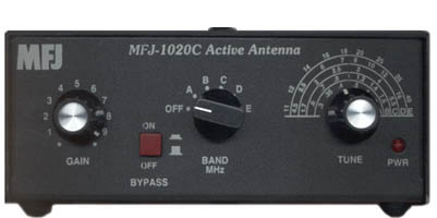The MFJ-1020C is a tunable preselector combined with an RF amplifier. Connect the antenna to the input of the preselector and connect the A/D input to its output. Set the GAIN control to maximum, the BYPASSswitch OFF, and the BAND switch to B. On the VI, turn the RF filter off and select the envelope detector. You should be able to select different stations by adjusting the TUNE control on the preselector.

Part 7: An AM Transmitter

Build an AM transmitter:		Starting with the ni_proc VI (or from scratch if you wish) construct an AM transmitter (i.e. x(t)=(1+ms(t))cos(2πfct)) for a carrier frequency (fc) of 250 kHz. Include a switch to select the modulating input (s(t)) to be either a 1 kHz sine wave or the A/D input.
Question 4:		Since the D/A converter output is from a sample and hold rather than a bandpass filter, the output will contain aliases at higher frequencies. If the output were a perfect sample/hold what would the output frequencies be and what would be the amplitude of each?
Test the transmitter:		Connect the D/A output to the scope. Note that the steps of the output are not perfectly flat. Assuming this is due to a first order lowpass system, estimate the time constant and use this estimate to revise your amplitude estimates from the previous question. Connect the D/A output to the spectrum analyzer. Examine the output and verify that the frequencies and amplitudes are consistent with your analysis.
Transmitting:		Connect one of the whip antennas to the D/A output. Since the whip is only a small fraction of the wavelength it will not be a very efficient radiator, so our range will be fairly short. Connect the other whip antenna to the spectrum analyzer and see if you can receive the signal. Using one of the Kaito portable radios (or any other AM radio you have available) try to receive the signal on one or more of its harmonics.